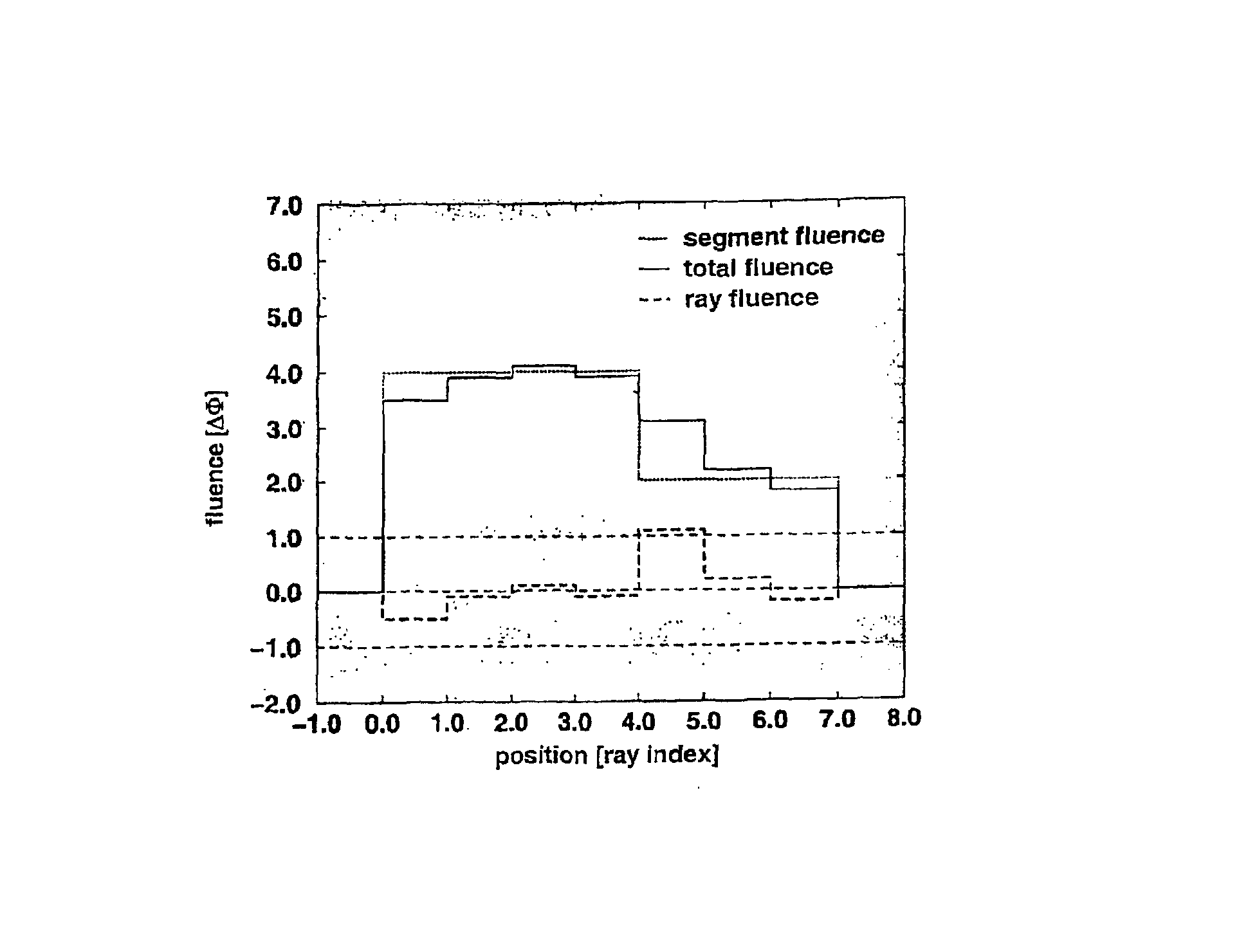
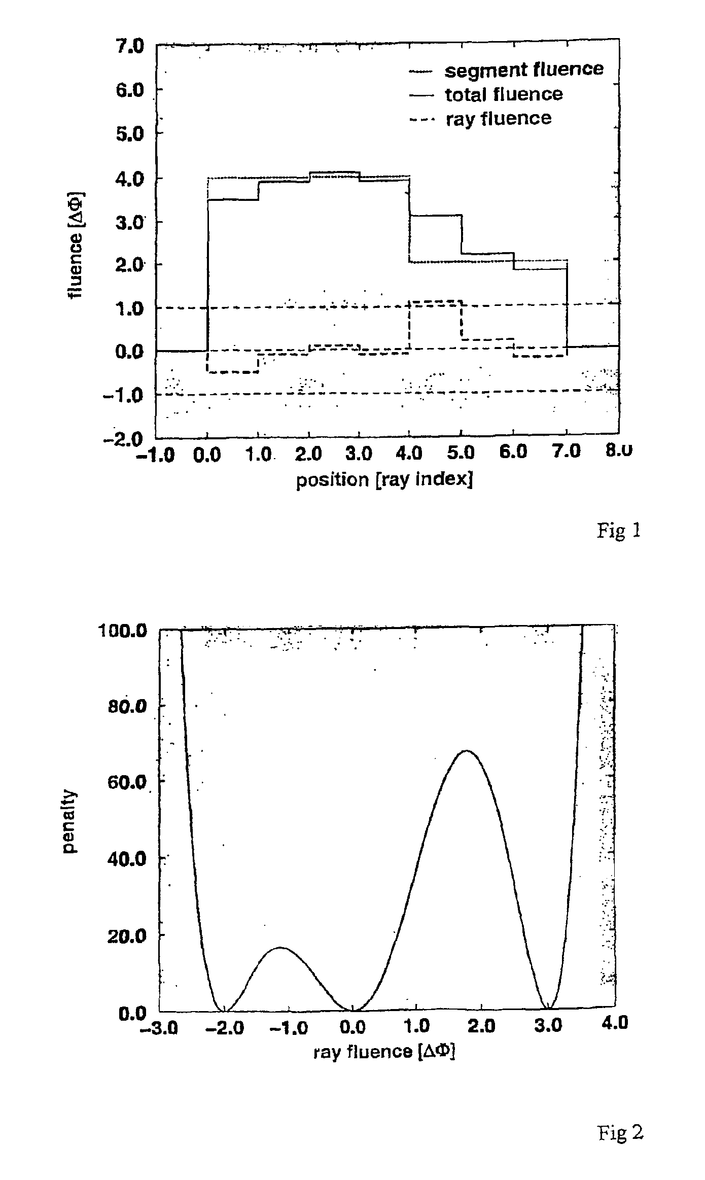
The setting of the optimisation problem is as follows. Let the fluence distribution φ(x,y) of a given field be composed of fluence elements termed rays Rij, i=1, . . . ,n, j=1, . . . ,m with fluence φij on a regular grid [ia, (i+1)a[x[jb, (j+1)b[for some real distances a, b. The positions of a pair of leafs at times t1, t2. . . can be described by coordinates with respect to the grid defined by the fluence elements. The total fluence of a ray is the ray fluence φij multiplied by the fluence weight φij.
The fluence distribution is translated by an operator P into a piecewise constant function with clusters of fluence elements of the same weight. These clusters result in a set of leaf coordinates and total fluences for each time tk such that this treatment plan is applicable with the given equipment. Such a pair of leaf coordinates and fluence is termed segment. This translation may be subject to complicated constraints related to the engineering details of the MLC. The hypothetic translator P groups the fluence elements such that the fluence distribution consists of the minimum number of stacked segments of maximum size.
If a number of fluence elements is exposed during the time interval [tk, tk+l] while the beam is on, this set of rays is called the segment Sk with total fluence ψk, see FIG. 1. To allow for an unambiguous correlation between segments and rays, we denote with Sij the smallest segment which contains the ray rij. Likewise, ψij denotes the total fluence of the profile which passes through the area delineated by the segment Sij. Notice that the fluence of these mathematical segments is not equivalent to the physical fluence passing through the field as delineated by the collimators.
We assume that the optimum fluence distribution can be obtained by minimising an objective function f(φ) with the property that if there exists one φij<0 then f(φ)=∞ to avoid negative fluence contributions. We assume further that f is a twice continuously differentiable function and does not possess local minima so that the minimum can be found with a fast gradient based algorithm.
There are several ways how the translation operator P can be used directly in conjunction with the optimisation algorithm to deliver an applicable fluence distribution (references 3 and 4). One way is to apply P to the optimum solution φ* a posteriori. While P may be constructed such that it does not overly deform the fluence distribution, this procedure does not grant any control over the dose distribution. It cannot be prevented that in some cases f(Pφ*)>>f(φ*).
Another way would be to feed Pφ* back into the optimisation and apply P regularly at particular iterations of the optimisation algorithm. This can cause erratic behaviour of the optimisation algorithm due to two effects. Firstly, the target set ⊂ of the operator P is non-convex. If we assume that this is the set of all piecewise constant fluence distributions with at most n fluence levels, then a convex combination of two elements can have up to 2n fluence levels, i.e. would not be an element of this set. As a consequence, the objective function will attain multiple local minima on . Secondly, the operator P is non-contracting, i.e. fluence distributions whose distance is small (e.g. as measured by the Euclidean norm) can be mapped onto fluence distributions which have a greater distance. This can cause an algorithm using gradient information to oscillate rather than converge.
To obtain a stable and consistent method of incorporating the MLC related constraints, two problems have to be solved. The parameter space over which f is minimised has to be convex, and the translation operator has to be contracting. This is achieved with the following modifications. 1. After each application of the operator P, the parameter space for the next iterations is composed of all rays Rij and all segments Sk, i.e. in the following iterations, the fluences of both segments and fluence elements are altered to minimise f. The barrier against negative fluences applies to the total local fluence, i.e. the sum of φij+ψij. With this alteration, the parameter space is convex, yet the fluence distribution is no longer unambiguously composed of ray fluences. 2. To provide for an unambiguous representation of the fluence distribution, a penalty term is introduced for all rays Rij which centers the fluence around 0
gij=φ2ij (1) Furthermore, for each neighbouring segment Si′,j′≠Sij, i′=i±1, j′=j±1, gij is multiplied with an additional term (φij+ψij−ψi′j′)2, so that gij is a polynomial of φij with a quadratic minimum at 0 and at each fluence increment to neighbouring segments, see FIG. 2. The sum g(φ) over all gij is added to f by means of a penalty multiplier λ to yield {circumflex over (ƒ)}
{circumflex over (ƒ)}(φij+ψij)=f(φij+ψk)+λ(φij) (2) where we stress the fact that the ψk are not considered as variables of g and are included into the optimisation only by means of f. Finding the feasible fluence which minimises f then becomes a two-tier problem. In an inner loop {circumflex over (ƒ)} is minimised, in an outer loop the operator P is applied to the result and the multiplier increased. With this arrangement, at high values of λ the ray fluences φij are forced to attain values such that the total fluence for ray Rij is either ψij or any of the neighbouring fluences ψi±1,j±1. At low values of λ the ray fluences may attain intermediate values. which show their tendency to smooth the edges of the segmented fluence distribution. Thus, the parameter λ can be seen as an inverse temperature: at high temperatures the ‘spins’φij may flip between ‘states’ψij, ψi±1,j±1; at low temperatures the spins ‘freeze out’ in either state representing the ‘ground state’. During the course of the optimisation λ is increased to reduce the ‘temperature’ of the fluence distribution. The role of the operator P is to mediate the transitions between states. 3. There is no translation operator for this problem which is generally contracting, but with the multistable penalty introduced above it is possible to condition the fluence distribution such that for this restricted problem a dedicated contracting translation operator can be devised. After the algorithm has converged for a given enlarged parameter space and a given penalty λ, the ray fluences contain information how the current segmenting may be improved. This incremental amendment of the segments prevents oscillation of the optimisation algorithm if the translation operator is fine-tuned to the problem. This can be achieved by a threshold Δφ for the minimum fluence increment between the segment and its surrounding segments; if the increment is below the threshold, the segment is concatenated with its neighbour. Likewise, new segments can only be created if the resulting fluence increment is above the threshold. The criteria according to which new segments are created or existing segments are altered may vary with the cost in terms of treatment time or monitor units incurred by these changes. Since the translation operator can alter, create and destroy segments, it cannot be generally non-contracting. However, it is contracting for all fluence distributions with ray fluences smaller than Δφ. Since all rays lying above the threshold are grouped into new segments if feasible, eventually the operator will always act on a fluence distribution for which it is contracting. This process is assisted, but not caused by the multistable penalty. The safe convergence was obtained at the cost of additional iterations. The number of segments depends on the threshold Δφ. The algorithm was described for the application of intensity modulated fields with a static MLC fields, a so-called step and shoot technique. The same fields may be applied while the beam is on leading to a dynamic close-in technique if the segments are arranged accordingly. Since the number of peaks in the fluence distribution can be controlled by the translation operator, it is often possible to derive unimodal fields (with a single peak) for which a dynamic close-in technique is the most efficient both in terms of monitor units and treatment time. Even for multimodal fluence distributions, a series of dynamic close-ins and leaf movements without irradiation may be favourable over other possibilities. For this general case the algorithm has to be slightly modified. Let jl be the position of the left leaf of pair i at time tk and jl+n be the position at time tk+1. The right leaf is at a position jrjl+n at both times. Let d(R) respectively d(S) be the dose at unit fluence from ray R respectively segment S. If the irradiation is interrupted during leaf travel, the segment dose consists of the sum of the rays d ( S k ) = ∑ i = 0 n - 1 d ( R i , j + 1 )
and segment dose d ( S k + 1 ) = ∑ i = 0 m - n - 1 d ( R i , j + n + i ) .
In case the irradiation is not interrupted, let the segment dose be composed of d ( S k ) = ∑ i = 0 n - 1 ( n - i ) / nd ( R i , j + i )
and segment dose d ( S k + 1 ) = ∑ i = 0 n - 1 i / nd ( R i , j + i ) + ∑ i = 0 m - n - 1 d ( R i , j + n + i ) .
The linear change of fluence between segment Sk and Sk+l corresponds to constant leaf velocity during time [tk, tk+l].
Results
The output of the algorithm are leaf positions and monitor units per MLC field, thus no translation errors can occur. The number of segments depends highly on the number of fields, the complexity of the treatment plan and the fluence increment threshold Δφ.
The example is a prostate case with overlapping PTV and rectum. The optimisation algorithm used biological constraints and a gradient technique, as per reference 5. The five fields were arranged in gantry angles of 0, 72, 144, 216 and 288 degrees. The resolution of the fluence distribution was 10×2 mm2 at the isocentre distance. The optimum treatment plan was computed without MLC constraints in about 10 minutes on a Pentium II/400 MHz and yielded an equivalent homogeneous dose to the PTV of 76.85 Gy. With inclusion of the translation operator, the fluence increment threshold was set to 5 MU which appears to be the lowest practical amount. The optimisation took 18 minutes and yielded a dose to the PTV of 76.55 Gy with a total of 39 segments. This marks a loss in target dose of less than 0.3 per cent. The target dose was subject to a homogeneity constraint so that we may conclude that the MLC constraint made the dose distribution less homogeneous, as can be seen from FIG. 3.
Of the five fields, two were unimodal and the remaining bimodal. The field from anterior oblique (72°) has five segments which can be applied with a minimum of leaf travel.
The field from posterior oblique (216°) has eight segments which can be separated into two leaf sweeps. As a consequence, a dynamic close-in technique would be advantageous for this case.
The number of segments is strongly dependent on the fluence increment threshold. If it is set to 10 MU, the same plan requires 27 segments at a loss of 0.5 per cent target dose. The number of segments could be reduced further if the beams were slightly rearranged such that the projection of the rectum aligns with the outline of the PTV. This measure would prove far more efficient than increasing the fluence increment threshold further.
Conclusion
The use of projection operators in iterative gradient based optimisation algorithms to ensure technical feasibility of the fluence profiles may lead to erratic behaviour and slow convergence. The strategy introduced here is to condition the fluence distribution such that the translation operator cannot disturb the convergence to an optimum and feasible solution. The method converges rapidly and allows to control the number of segments. For some treatment cases the number of segments may be as low as 20 without loss in the quality of the dose distribution. With few and relatively large field segments, IMRT becomes a viable alternative to standard treatment techniques.
References 1 M. Alber and F Nússlin, “Intensity modulated photon beams subject to a miminal surface smoothness constraint”Phys Med Biol, 45:N49-N52, 2000 2 S. Webb, D. J. Convery and P. M. Evans, “Inverse planning with constraints to generate smoothed intensity-modulated beams”, Phys Med Biol., 43:2785-2794, 1998 3 M- A. Keller-Reichenbecher, T. Bortfeld, S. Levegrún, J. Stein, K. Preiser and W. Schlegel, “Intensity modulation with the ‘step and shoot’ technique using a commercial mic: a planning study”, Int. J. Rad. Oncol. Biol. Phys., 45:1315-1324, 1999 4 P. S. Cho and R. J. Marks, “Hardware-sensitive optimisation for intensity modulated radiotherapy”, Phys. Med. Biol., 45:429-440, 2000 5 M. Alber, M. Birkner, W. Laub and F. Nússlin, “Constrained biological optimisation of imrt”, submitted to Phys. Med. Biol., 2000