Integrated calibration method for gyro and magnetic transducer

A magnetic sensor and joint calibration technology, applied in the field of sensors, can solve the problems of affecting the calibration effect of magnetometer and gyroscope, large bias error of low-cost gyroscope, inability to calibrate magnetometer, etc.

Active Publication Date: 2016-05-04
SHANGHAI JIAO TONG UNIV
5 Cites 9 Cited by

AI-Extracted Technical Summary

Problems solved by technology

The commonly used magnetometer calibration method takes advantage of the fact that the local magnetic field strength has nothing to do with the attitude of the magnetometer. The advantage is that no external auxiliary equipment is required, and the disadvantage is that it cannot calibrate the misalignment angle of the coordinate system between the magnetometer and ot...

Abstract

The invention provides an integrated calibration method for a gyro and a magnetic transducer. The method is characterized by comprising the following steps: step 1, obtaining an associated measuring model of the magnetic transducer and the gyro, wherein the measuring model includes a calibration parameter; and step 2, adopting constraint non-linear least square estimation based on the calibration parameter to obtain a determined value of the calibration parameter. Compared with a method in the prior art, the integrated calibration method has the following beneficial effects: 1, both a misalignment angle between the magnetic transducer and the gyro and a gyro zero offset are calibrated; 2, in a calibration process, the more stable the magnetic field is, the better the calibration effect is, and the calibration effect is not interfered by any accelerated speed, so that the gyro and the magnetic transducer do not need to be kept in a stationary state; and 3, the method can be used for attitude rectification of the magnetic transducer and an inertia measuring unit (including the gyro and an accelerometer).

Application Domain

Measurement devices

Technology Topic

PhysicsInertial measurement unit +8

Image

  • Integrated calibration method for gyro and magnetic transducer
  • Integrated calibration method for gyro and magnetic transducer
  • Integrated calibration method for gyro and magnetic transducer

Examples

  • Experimental program(1)

Example Embodiment

[0045] The present invention will be described in detail below with reference to specific embodiments. The following examples will help those skilled in the art to further understand the present invention, but do not limit the present invention in any form. It should be noted that, for those skilled in the art, several changes and improvements can be made without departing from the inventive concept. These all belong to the protection scope of the present invention.
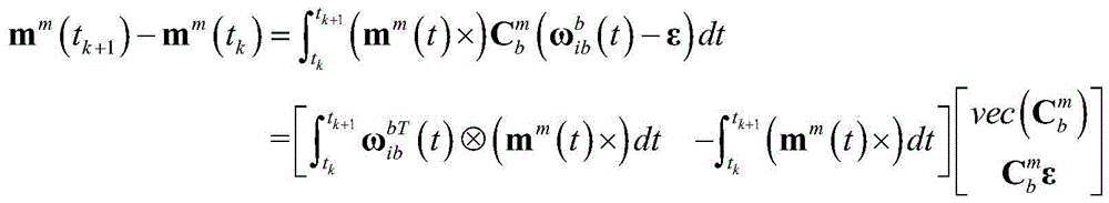
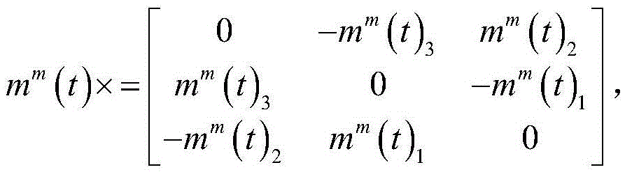
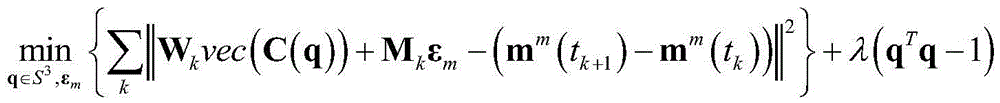
[0046]In a stable magnetic field, the change of the measured value of the three-axis magnetic sensor is entirely caused by the change of attitude. Based on this fact, the present invention provides a joint calibration method for the misalignment angle of the coordinate system between the three-axis magnetometer and the three-axis gyro and the zero offset of the gyro. The magnetometer and the gyroscope are fixedly connected, and the attitude is fully changed and the measurements of the magnetometer and the gyroscope are collected synchronously. The magnetometer data can be used for the internal calibration of the magnetometer, and the data of the magnetometer and the gyroscope are jointly used for the joint calibration of the misalignment angle of the coordinate system between the magnetometer and the gyroscope and the zero offset of the gyroscope of the present invention. The following assumes that the magnetometer internal calibration has been implemented.
[0047] The joint calibration method of the gyroscope and the magnetic sensor of the present invention includes: obtaining an associated measurement model of the magnetic sensor and the gyroscope, wherein the measurement model includes parameters such as the misalignment angle of the coordinate system and the zero bias of the gyroscope; The square estimation obtains the determined value of the calibration parameter.
[0048] Among them, the correlation measurement model is:
[0049] m m ( t k + 1 ) - m m ( t k ) = ∫ t k t k + 1 ( m m ( t ) × ) C b m ( ω i b b ( t ) - ϵ ) d t = [ ∫ t k t k + 1 ω i b b T ( t ) ⊗ ( m m ( t ) × ) d t - ∫ t k t k + 1 ( m m ( t ) × ) d t ] v e c ( C b m ) C b m ϵ
[0050] where m m (t k+1 ) represents the k+1th time t k+1 The magnetic field vector in the magnetic sensor coordinate system m, m m (t k ) represents the kth time t k is the magnetic field vector in the magnetic sensor coordinate system m, k is a positive integer, m m (t) represents the magnetic field vector in the magnetic sensor coordinate system m at time t, represents the misalignment matrix of the magnetic sensor and the gyro coordinate system, Represents the angular velocity vector of the gyro coordinate system b at time t, ε represents the zero bias vector of the gyro; vec( ) means that the matrix is ​​spliced ​​in the order of the columns;
[0051] m m (t)×represented by the three-dimensional vector m m (t)=[m m (t) 1 m m (t) 2 m m (t) 3 ] T The cross-product matrix formed, that is m m ( t ) × = 0 - m m ( t ) 3 m m ( t ) 2 m m ( t ) 3 0 - m m ( t ) 1 - m m ( t ) 2 m m ( t ) 1 0 , where m m (t) 1 Represents the component in the X direction of the magnetic field vector in the magnetic sensor coordinate system m at time t; where m m (t) 2 Represents the component in the Y direction of the magnetic field vector in the magnetic sensor coordinate system m at time t; where m m (t) 3 Represents the Z-direction component of the magnetic field vector in the magnetic sensor coordinate system m at time t.
[0052] Preferably, the constrained nonlinear least squares estimate is derived from the correlation measurement model:
[0053] min q ∈ S 3 , ϵ m { Σ k | | W k v e c ( C ( q ) ) + M k ϵ m - ( m m ( t k + 1 ) - m m ( t k ) ) | | 2 } + λ ( q T q - 1 )
[0054] Among them, S 3 Represents a four-dimensional vector modulo 1; λ is the Lagrangian coefficient; q=[q 0 q 1 q 2 q 3 ] T is the misalignment matrix of the magnetic sensor and the gyro coordinate system the corresponding quaternion, q 0 ,q 1 ,q 2 ,q 3 Represent the four components of the quaternion q, and the quaternion q is represented as q 0 +q 1 i+q 2 j+q 3 k, where the imaginary units i, j, and k satisfy the operation rules: i 0 =j 0 =k 0 =1,i 2 =j 2 =k 2 =-1;ε m represents the zero bias of the gyro in the magnetic sensor coordinate system, ϵ m = C b m ϵ ;
[0055] C ( q ) = q 0 2 + q 1 2 - q 2 2 - q 3 2 2 ( q 1 q 2 + q 0 q 3 ) 2 ( q 1 q 3 - q 0 q 2 ) 2 ( q 1 q 2 - q 0 q 3 ) q 0 2 - q 1 2 + q 2 2 - q 3 2 2 ( q 2 q 3 + q 0 q 1 ) 2 ( q 1 q 3 + q 0 q 2 ) 2 ( q 2 q 3 - q 0 q 1 ) q 0 2 - q 1 2 - q 2 2 + q 3 2 ;
[0056] vec(C(q)) means splicing the matrix C(q) in the order of columns;
[0057] The coefficient matrix W of the misalignment attitude matrix between the magnetic sensor and the gyro coordinate system k for:
[0058] W k = ∫ t k t k + 1 ω i b b T ( t ) ⊗ ( m m ( t ) × ) d t ;
[0059] The coefficient matrix M of the zero bias of the gyro k for:
[0060] M k = - ∫ t k t k + 1 ( m m ( t ) × ) d t ;
[0061] m m (t)×represented by the three-dimensional vector m m (t)=[m m (t) 1 m m (t) 2 m m (t) 3 ] T The cross-product matrix formed, that is m m ( t ) × = 0 - m m ( t ) 3 m m ( t ) 2 m m ( t ) 3 0 - m m ( t ) 1 - m m ( t ) 2 m m ( t ) 1 0 , where m m (t) 1 Represents the component in the X direction of the magnetic field vector in the magnetic sensor coordinate system m at time t; where m m (t) 2 Represents the component in the Y direction of the magnetic field vector in the magnetic sensor coordinate system m at time t; where m m (t) 3 Represents the Z-direction component of the magnetic field vector in the magnetic sensor coordinate system m at time t.
[0062] Preferably, the initial value of the misalignment attitude matrix of the magnetic sensor and the gyro coordinate system is obtained from the associated measurement model by using the linear least squares method and the initial value of the gyro bias
[0063] v e c ( C b m ) ϵ m = ( Σ k W k M k T [ W k M k ] ) - 1 Σ k W k M k T ( m m ( t k + 1 ) - m m ( t k ) ) ;
[0064] from the least squares solution to extract the corresponding and Will Orthogonalize and use the transformation relationship between the attitude matrix and the quaternion to obtain the initial value q of the quaternion (0) , the initial value of the Lagrangian coefficient λ (0) Set to zero.
[0065] Preferably, the calculation is iterative until the convergence conditions are met:
[0066] x ( i + 1 ) = x ( i ) - [ H | x ( i ) ] - 1 J | x ( i ) , i = 0 , 1 , ... ;
[0067] where x (i+1) Indicates the i+1th iteration value of the parameter x to be estimated, x (i) Indicates the ith iteration value of the parameter x to be estimated, J is the Jacobian matrix derivative vector, H is the Hessian matrix, and the parameter x to be estimated is:
[0068] x = q T ϵ m T λ T ;
[0069] Among them, the Jacobian matrix derivative vector J and the Hessian matrix H are:
[0070] J = J q T J ϵ m T J λ T
[0071] H = H q q H qϵ m H q λ H qϵ m T H ϵ m ϵ m 0 3 × 1 H q λ T 0 3 × 1 T 0
[0072] in,
[0073] J q = 2 λ q + 2 Σ k ∂ q T ( v e c ( C ( q ) ) ) W k T α k , J ϵ m = 2 Σ k M k T α k , J λ =q T q-1,
[0074] H q q = 2 λI 4 + 2 Σ k { ∂ q T ( v e c ( C ( q ) ) ) W k T W k ∂ q ( v e c ( C ( q ) ) ) + Q 0 T W k T α k Q 1 T W k T α k Q 2 T W k T α k Q 3 T W k T α k T } ,
[0075] H qϵ m = 2 Σ k ∂ q T ( v e c ( C ( q ) ) ) W k T M k ,
[0076] H q λ = 2 q , H ϵ m ϵ m = 2 Σ k M k T M k
[0077] alpha k =W k vec(C(q))+M k ε m -(m m (t k+1 )-m m (t k )),
[0078] ∂ q ( v e c ( C ( q ) ) ) = 2 q 0 q 1 - q 2 - q 3 - q 3 q 2 q 1 - q 0 q 2 q 3 q 0 q 1 q 3 q 2 q 1 q 0 q 0 - q 1 q 2 - q 3 - q 1 - q 0 q 3 q 2 - q 2 q 3 - q 0 q 1 q 1 q 0 q 3 q 2 q 0 - q 1 - q 2 q 3 ,
[0079] Q 0 = 1 0 0 0 0 0 0 - 1 0 0 1 0 0 0 0 1 1 0 0 0 0 - 1 0 0 0 0 - 1 0 0 1 0 0 1 0 0 0 , Q 1 = 0 1 0 0 0 0 1 0 0 0 0 1 0 0 1 0 0 - 1 0 0 - 1 0 0 0 0 0 0 1 1 0 0 0 0 - 1 0 0 , Q 2 = 0 0 - 1 0 0 1 0 0 1 0 0 0 0 1 0 0 0 0 1 0 0 0 0 1 - 1 0 0 0 0 0 0 1 0 0 - 1 0 , Q 3 = 0 0 0 - 1 - 1 0 0 0 0 1 0 0 1 0 0 0 0 0 0 - 1 0 0 1 0 0 1 0 0 0 0 1 0 0 0 0 1 .
[0080] Specific embodiments of the present invention have been described above. It should be understood that the present invention is not limited to the above-mentioned specific embodiments, and those skilled in the art can make various changes or modifications within the scope of the claims, which do not affect the essential content of the present invention. The embodiments of the present application and features in the embodiments may be combined with each other arbitrarily, provided that there is no conflict.

PUM

no PUM

Description & Claims & Application Information

We can also present the details of the Description, Claims and Application information to help users get a comprehensive understanding of the technical details of the patent, such as background art, summary of invention, brief description of drawings, description of embodiments, and other original content. On the other hand, users can also determine the specific scope of protection of the technology through the list of claims; as well as understand the changes in the life cycle of the technology with the presentation of the patent timeline. Login to view more.
Why Eureka
Try Eureka