[0046] The present invention will be further described in detail below with reference to the drawings and embodiments. This embodiment is a 750kV line project in a certain area of Xinjiang, with a design wind speed of 31m/s (10m high in 50 years, 10min average maximum), ice coating 5mm, and extreme minimum temperature -30.0°C.
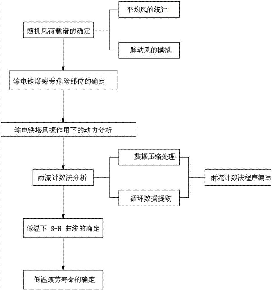
[0047] Such as figure 1 As shown, the steps of the method for predicting the fatigue life of transmission towers in cold regions are: determination of random wind load spectrum→determination of dangerous parts of the transmission tower→dynamic analysis under wind vibration of transmission tower→analysis of rain flow counting method→SN curve at low temperature Determination of → determination of low-temperature fatigue life, the specific process is as follows:
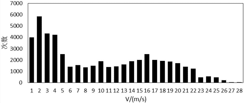
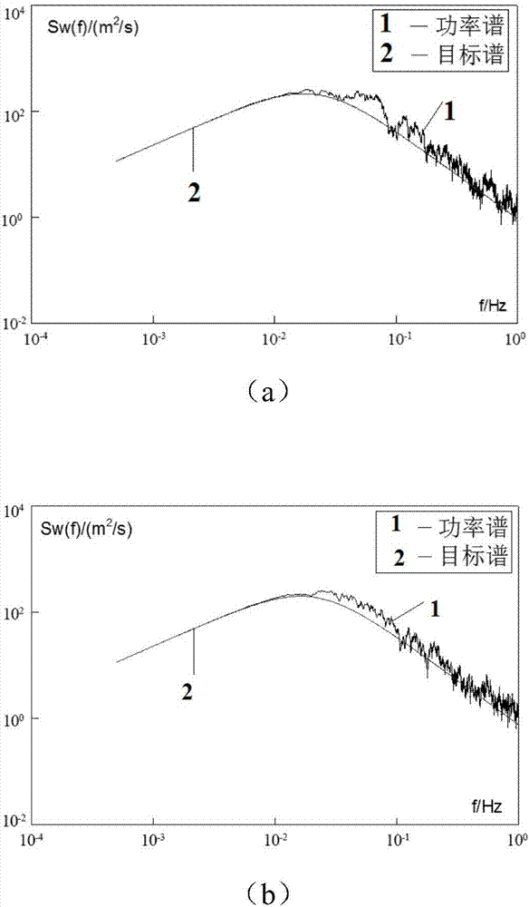
[0048] 1) Determination of random wind load spectrum: The average wind and fluctuating wind in the cold area are calculated and simulated respectively, and the average wind speed distribution map and fluctuating wind speed time history curve of 10m high and 10min in the cold area are obtained, and then the average wind speed distribution map The average wind speed at each point is added to the fluctuating wind speed time history curve to obtain the instantaneous wind speed at each point in the space, and the instantaneous wind speed is converted into wind load to obtain the wind load time history. The wind load at each point is loaded on the transmission tower as External input conditions;
[0049] Among them, (1) The statistics of the average wind in cold areas are measured by meteorological stations, which is the average wind speed of 10m in height and 10min in cold areas In this example, the 10m high 10min average wind speed distribution diagram of a 750kV line project in a certain area of Xinjiang is as follows figure 2 Shown
[0050] (2) The simulation of fluctuating wind in cold areas is carried out by the improved Iwatani linear regression filter method. The solution of fluctuating wind speed v(t) in cold areas includes:
[0051] ① Find the regression coefficient
[0052] The AR method is used to extend the technology to simulate the multi-dimensional wind speed process. The random processes of M related winds are:
[0053] [u(t)]=[u 1 (t),...u M (t)] T (1)
[0054]
[0055] In formula (2): [u(t-kΔt)]=[u 1 (t-kΔt),…,u M (t-kΔt)] T;
[0056] [N(t)]=[N 1 (t),…,N M (t)], N i (t) is a normal distributed random process with a mean value of 0 and a given covariance, i=1,...,M; [Ψ k ] Is an M×M order matrix, k=1,...,p.
[0057] For any point i (i=1,...,M) in a random process with time difference, u in formula (1) i (t) and u in formula (2) i The covariance of (t-kΔt) can be expressed as:
[0058]
[0059] Because u i (t) and u i (t-kΔt) is a stable random wind process with a mean value of 0, and the value of its covariance is only a function of the time difference. Equation (3) can be rewritten as:
[0060]
[0061] Equation (4) right multiplying [u(t-kΔt)]=[u(t)]=[u 1 (t-kΔt),...u M (t-kΔt)] T , Taking the mathematical expectation on both sides at the same time, considering that the mean of [N(t)] is 0, and it is related to the random process u i (t) independence, and covariance R u (jΔt) is an even function, the covariance R can be obtained u (jΔt) and regression coefficient [Ψ k ] The relationship between, written in matrix form, can be expressed as:
[0062]
[0063] In the formula, [R] pM×M =[R u (Δt),…,R u (pΔt)] T;
[0064]
[0065] among them,
[0066]
[0067]
[0068] According to the random vibration theory, the power spectral density and the correlation function (covariance) conform to the Wiener-Khintchine formula, namely:
[0069]
[0070] Solving the linear equations given by equation (5), the regression coefficient matrix [Ψ] can be obtained.
[0071] ②The random process of finding the given variance [N(t)]
[0072] Equation (2) right multiplication [u(t)]=[u 1 (t),...u M (t)], which can be expressed as:
[0073]
[0074] Find [R N ] After the [R N ] Do Cholesky decomposition [R N ]=[L][L] T , The random process of given variance [N(t)]=[L][n(t)] (11)
[0075] Among them, n(t)=[n 1 (t),n 2 (t),…,n M (t)], n i (t) is a normal random process with a mean value of 0, a variance of 1 and independent of each other, i=1,...,M.
[0076] ③ Solve the final M random processes
[0077] Find the regression coefficient matrix [Ψ] and [R N ] Then, according to equation (2), M spatially related random wind processes are solved, and equation (2) is discretized according to the time interval Δt. Assuming t<0, u i (t) = 0, the recursive matrix expression is:
[0078]
[0079] Thus, M discrete pulsating wind speed time history vectors with time, space correlation and time interval Δt are obtained, that is, the pulsating wind speed v(t) in cold areas.
[0080] (3) Instantaneous wind speed V(t) at each point in the cold area
[0081]
[0082] In formula (13) It is the average wind speed of 10m high and 10min in the cold area, and v(t) is the pulsating wind speed.
[0083] (4) Wind load borne by the transmission tower
[0084] The wind load borne by the transmission tower is formed by the combined action of static wind and dynamic wind. In this example, the average wind speed is 10m high and 10min high in cold areas. The resulting average wind load and the fluctuating wind load of the fluctuating wind speed v(t) in cold areas are integrated into the instantaneous wind load.
[0085] ① 10m high 10min average wind speed in cold areas The resulting average wind load:
[0086] According to the classical wind load theory, the average wind speed of 10m high and 10min in the cold area Average wind load on the structure Expressed as:
[0087]
[0088] In formula (14), w 0 Is based on the basic wind speed in the area where the building is located Calculated basic wind load; μ r Is the return period adjustment factor; μ s Is the structural body shape coefficient; μ z Is the wind load height variation coefficient.
[0089] ②Fluctuating wind load w of fluctuating wind speed v(t) in cold regions f :
[0090] Set any instantaneous wind load at any height as w, and consider the fluctuating wind speed v(t)(v f ) And average wind speed Compared to it is much smaller, the fluctuating wind load w can be obtained f Variance for:
[0091]
[0092] From the properties of the Gaussian stationary process with zero mean:
[0093]
[0094]
[0095] And from this, the power spectrum of the fluctuating wind load S wf (z, f) and fluctuating wind speed spectrum S v The relationship between (f) is:
[0096]
[0097] Set fluctuating wind load w f Can be decomposed into functions of position and time:
[0098] w f (z,f)=w f (z)f(t) (19)
[0099] Because of fluctuating wind load w f Is a random load, so w f (z) should be substituted with statistical values, that is, the mean square error σ wf (z) is substituted, and f(t) has a normalized power spectrum (ie ), then the fluctuating wind load power spectrum S wf (Z, f) can be expressed as:
[0100]
[0101] In practical applications, the design fluctuating wind speed is taken as the mean square error of fluctuating wind load σ wf Multiplied by the guarantee factor μ (μ=2.0-2.5), our country's load code is μ=2.2 (guarantee rate 98.61%), it is recommended to adopt:
[0102]
[0103] Therefore, the mean square error of the fluctuating wind load at the structure height z is:
[0104]
[0105] According to observations of strong winds, the wind speed and wind direction at various points on the windward surface of the structure are not completely synchronized, and some are even almost irrelevant. For this reason, the pulsating wind load on the building structure must consider its spatial correlation. For three-dimensional problems, the correlation function generally has the following form:
[0106]
[0107] In formula (23), C x , C y , C z Is the attenuation coefficient, determined by experiment.
[0108] ③ Instantaneous wind speed power spectrum in cold areas
[0109] Combined with the statistical parameter values of the above random process simulation, the instantaneous wind speed power spectrum S is obtained according to the following general power spectrum expression of instantaneous wind speed proposed by Davenport v (f):
[0110]
[0111] In formula (24): f is the frequency (Hz).
[0112] In this example, the average wind speed of 10m high and 10min in a cold environment where a 750kV line project in a certain area of Xinjiang is located The instantaneous wind speed power spectral density at image 3 As shown, the spectral line trend of the instantaneous wind speed power spectrum simulated for the tower top, tower body, and tower bottom is consistent with the target spectrum, and the overall mean value of the spectrum is also very close to the target spectrum, indicating the pulsation used in the present invention The wind simulation method and the selected parameters are reasonable.
[0113] ④ Instantaneous wind load in cold areas
[0114] The calculation formula for the instantaneous wind load F of the transmission tower body is as follows:
[0115]
[0116] In formula (25): v is the instantaneous wind speed, μ s Is the wind load carrier shape coefficient, and A is the sum of the projected area of the windward side members in a plane perpendicular to the wind direction.
[0117] 2) Determination of the fatigue dangerous parts of the transmission tower: Use the wind load time history obtained in step 1) to perform a finite element analysis on the transmission tower, and then determine the fatigue risk parts of the transmission tower structure according to the structural characteristics of the transmission tower and the results of the finite element analysis , Where the fatigue dangerous parts are determined as dangerous tension members and welds, and the component units of the dangerous parts are selected as Figure 4 As shown, it includes No. 61 component unit, No. 274 component unit, No. 595 component unit, No. 611 component unit, No. 671 component unit and No. 673 component unit;
[0118] 3) Dynamic analysis under wind vibration of the transmission tower: add the wind load time history obtained in step 1) to the nodes of the transmission tower for time history calculation, and then perform stress analysis on the fatigue risk parts in step 2) to obtain the Stress spectrum, and extract the stress time history curve and stress amplitude level under different wind loads. Among them, the average wind speed of 10m high and 10min in the cold environment of a 750kV line project in a certain area of Xinjiang in this example The stress time history curve of No. 673 component element at time is as Figure 5 Shown
[0119] 4) Rain flow counting method analysis: According to the stress time history curve under different wind loads in step 3), the rain flow counting method is used to count the stress amplitude of the fatigue dangerous parts in step 2) and the number of occurrences of each stress amplitude;
[0120] Among them, the specific steps of using rainflow counting method to analyze are:
[0121] (1) Data compression processing: including equal interval sampling, elimination of false readings, peak and valley value detection and invalid amplitude removal;
[0122] (2) Cyclic data extraction: According to the skew waveform, it is completed in three steps: primary rain flow counting, docking and secondary rain flow counting;
[0123] (3) Use MATLAB to compile the rain flow counting method program. The whole program includes eight subroutines and a calling program.
[0124] In this example, the average wind speed of 10m high and 10min in a cold environment where a 750kV line project in a certain area of Xinjiang is located The rain flow statistics of No. 673 component unit at time Image 6 Shown.
[0125] 5) Determination of the S-N curve at low temperature: According to the stress amplitude of the fatigue risk part in step 2) obtained in step 4), the S-N curve of the fatigue risk part in step 2) at low temperature is obtained through the constant stress amplitude test;
[0126] Among them, the constant stress amplitude test is realized by the cooperative work of MTS electro-hydraulic servo testing machine and low-temperature test box. It uses MTS electro-hydraulic servo testing machine and low-temperature test box to conduct the test pieces (plates and weldments) at room temperature, 0℃,- Axial cyclic tensile fatigue test under different temperature conditions of 15°C and -30°C, thereby obtaining and drawing the fatigue characteristic curves of test pieces (plates and weldments) at different temperatures, namely the SN curve, the SN curve In order to obtain the stress amplitude S of the test piece (plate and weldment) at low temperature through the equal stress amplitude test i And the number of cycles N i The relationship curve of S-N curve is expressed by a power function formula.
[0127] The fatigue characteristic curves of the test pieces (plates and weldments) in the present invention at room temperature, 0°C, -15°C, -30°C are as follows Figure 7~10 As shown, and the present invention uses the linear regression method to fit the test data in the fatigue characteristic curve, and then uses the least square method to determine the regression coefficient, and the fatigue performance parameters of the obtained test pieces (plates and weldments) are shown in Table 1 and Table 2 shows, where, Figure 7 The selected test piece is Q420B steel plate, Figure 8 The selected test piece is Q420C steel plate, Picture 9 The selected test piece is Q420B steel weldment, Picture 10 The selected test piece is Q420C steel weldment. In Table 1, A=lgC/m, B=-(1/m).
[0128] Table 1
[0129]
[0130]
[0131] Table 2
[0132]
[0133] 6) Determination of low-temperature fatigue life: Apply the Miner linear cumulative damage theory and according to the number of cycles of fatigue dangerous parts on the SN curve in step 5) when they fail at low temperature and the number of times each stress amplitude of the fatigue dangerous parts in step 4) appears, Obtain the damage rate generated by the stress amplitude level under different wind loads in step 3), and accumulate the damage rate. When the cumulative damage rate reaches 1, the fatigue risk part fails. Then, according to the annual accumulation of fatigue risk part The damage rate can obtain the low-temperature fatigue life of the fatigue-dangerous parts.
[0134] The cumulative damage rate D of the selected component unit in this embodiment can be expressed as:
[0135]
[0136] In formula (26), n i The number of occurrences of each stress amplitude of the component unit selected in this embodiment, N i The number of cycles when the component unit selected for this embodiment is broken at low temperature.
[0137] The low temperature fatigue life T of the component unit selected in this embodiment can be expressed as:
[0138] T = 1/D T (27)
[0139] In formula (27), D T Is the cumulative damage rate throughout the year, which is the sum of the cumulative damage rate D.
[0140] In this embodiment, the specifications and lifespan of the six component units selected on the transmission tower of a 750kV line project in a certain area of Xinjiang are shown in Table 3. Table 3 shows that the fatigue life of the transmission tower of a 750kV line project in a certain area of Xinjiang is 62.8 years.
[0141] table 3
[0142]
[0143] The parts not described in detail in the present invention belong to the prior art.