Escalator passenger detection algorithm based on fast Adaboost training algorithm

[0108] The present invention will be further described below in conjunction with specific embodiments.

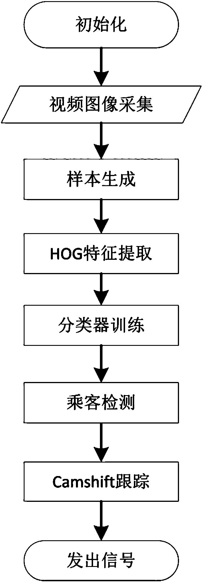
[0109] Such as figure 1 As shown, the escalator passenger detection algorithm based on the fast Adaboost training algorithm provided in this embodiment mainly collects video samples, extracts HOG features, quickly trains to obtain a classifier, and uses the classifier to detect passengers on the escalator. In this algorithm, the area of ​​interest is the passenger area of ​​the escalator. Therefore, the camera is installed diagonally above the escalator movement direction. The specific conditions are as follows:

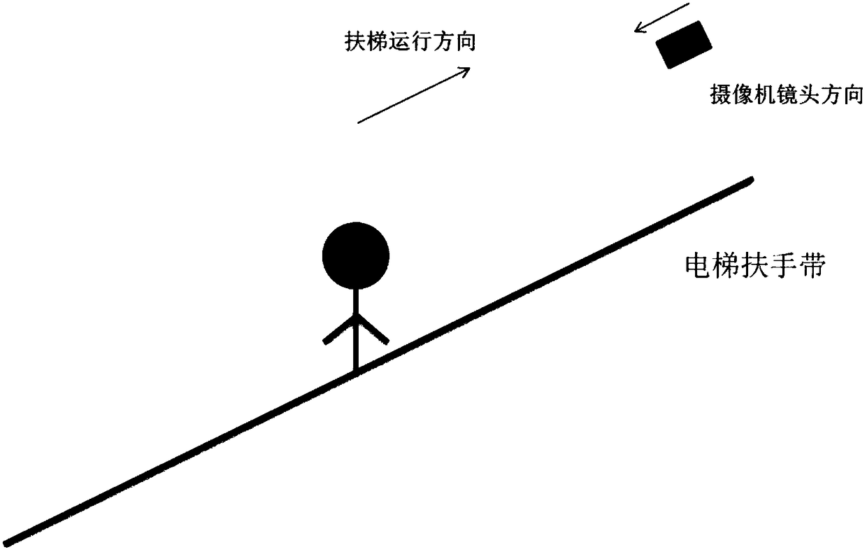
[0110] 1) The camera is used for image acquisition. The camera is installed obliquely above the moving direction of the escalator. Its viewing angle is required to cover the entire escalator passenger area and ensure that the passengers on the escalator are in the middle of the video, see figure 2. The camera used is specifically a PAL standard-definition camera with a pixel of 640*480, and 30 frames of image data are collected per second. For the images captured by the camera, see image 3.

[0111] 2) After obtaining the original video, intercept the positive and negative samples, including the following steps:

[0112] 2.1) Obtain a positive sample

[0113] Save the collected video frame by frame into an image sequence, and the total number of original images is N origin; In the obtained picture, the rectangular image containing the complete human body is intercepted frame by frame, and the total number of positive sample images is N pos; Normalize all rectangular images to a standard rectangular image with a pixel in length and b pixel in height; number all positive sample images and attach the sample label corresponding to the number to complete the generation of positive samples. The positive sample image of Yihua see Figure 4a;

[0114] In this embodiment, the total number of original images N origin Is 4000, the total number of positive sample images N pos It is 2000, the length of the positive sample image is 64 pixels, and the height is 128 pixels.

[0115] 2.2) Get negative samples

[0116] Save the collected video as an image sequence frame by frame, and remove the human body images contained therein; cut out the sample images from the remaining images according to the length to height ratio of a:b, and the total number of negative sample images is N neg; Number all negative sample images and attach the sample label corresponding to the number to complete the negative sample generation.

[0117] In this embodiment, the total number of negative sample images N neg Is 2000, the length of the negative sample image is 64 pixels, and the height is 128 pixels. For the unnormalized negative sample image, see Figure 4b.

[0118] 3) Extracting HOG features in positive and negative samples includes the following steps:

[0119] 3.1) Grayscale

[0120] According to the importance and other indicators, the three components are weighted and averaged with different weights; since the human eye is the most sensitive to green and the least sensitive to blue; therefore, the weighted average of the three components of RGB can be obtained by the following formula. Reasonable grayscale image:

[0121] I(x,y)=0.30R(x,y)+0.59G(x,y)+0.11B(x,y)

[0122] Where x, y are the abscissa and ordinate of a pixel in the image; I (x, y) is the gray value of the image midpoint (x, y); R (x, y) is the image midpoint (x, y) the red component brightness; G(x,y) is the green component brightness of the point (x,y) in the image; B(x,y) is the blue component brightness of the point (x,y) in the image;

[0123] Calculate the gray value of all pixels in the image in turn to complete the grayscale of the image;

[0124] 3.2) Gamma correction

[0125] In order to suppress the illumination changes in the image; Gamma compression is performed on the image, the Gamma compression formula is:

[0126] I(x,y)=I(x,y) Gamma

[0127] Gamma is a fixed constant;

[0128] In this embodiment, selecting Gamma as 2000 can achieve a better compression effect.

[0129] 3.3) Calculate the gradient of each pixel of the image

[0130] In order to capture contours, human shadows and some texture information, and further weaken the influence of lighting, it is necessary to calculate the gradient of the image's abscissa and ordinate directions, and calculate the gradient direction value of each pixel position accordingly; set the horizontal edge operator to [-1 01], the vertical edge operator is [-1 0 1] T , Then the direction gradient of the pixel I(x,y) is:

[0131] G x (x,y)=-I(x-1,y)+I(x+1,y)

[0132] G y (x,y)=-I(x,y-1)+I(x,y+1)

[0133] Where G x (x,y) is the horizontal gradient, G y (x,y) is the vertical gradient, then the gradient of pixel I(x,y) is:

[0134]

[0135]

[0136] Where G(x,y) is the magnitude of the gradient, and α(x,y) is the direction of the gradient.

[0137] 3.4) Image segmentation

[0138] In order to facilitate the subsequent operations, first divide the image into multiple cells; where the cell is a c×c image block as the basic unit of processing; c is the side length of the image block, and the unit is pixel;

[0139] In this embodiment, the cell size is selected as 8×8.

[0140] 3.5) Construct a histogram of gradient directions

[0141] In order to count and quantify the local image gradient information, obtain the feature description vector of the local image area; at the same time, it can maintain the weak sensitivity to the posture and appearance of the human object in the image; it is necessary to construct a gradient direction histogram for each cell;

[0142] Use N bin The histogram of each direction counts the gradient information of a cell, which is equivalent to dividing the gradient direction of the cell by 360° into N bin Direction blocks. Use the gradient magnitude as the weight to vote for each direction block, and get the direction histogram of the cell. The abscissa is 360° divided into N bin The angle interval of the part, the pixel gradient of the ordinate is the number that falls into the interval; at this time, each cell corresponds to a N bin Dimensional feature vector;

[0143] In this embodiment, the number of angle intervals N bin Selected as 9.

[0144] 3.6) Normalization of gradient intensity

[0145] In order to reduce the influence of local illumination changes and foreground and background contrast, and reduce the range of gradient intensity, it is necessary to normalize the gradient intensity;

[0146] Combine n cells into a larger, spatially connected block; the feature vectors of all cells in a block are concatenated to be the HOG feature vector of the block; the feature of each cell will have a different result It appears in the final feature vector multiple times; the normalized feature vector (block descriptor) is called HOG feature (HOG descriptor);

[0147] The normalization function is as follows:

[0148]

[0149] Where ν is the HOG feature vector of a block, ||v|| 2 It is the 2 norm of ν, and ε is a positive number less than 0.01, avoiding the denominator being 0;

[0150] In this embodiment, the number n of cells constituting the block is selected as 4, and ε is selected as 10. -5.

[0151] 3.7) HOG feature extraction

[0152] The length of the training sample is l and the height is h; the size of the feature scan window is the size of the block (n c×c image blocks), and the moving step is the side length c of the cell; the scan window starts from the vertex of the image , Perform scanning extraction. After each extraction, move one step in the horizontal direction and repeat the extraction process. When the scanning window touches the image boundary, move one step in the vertical direction, and continue to repeat the extraction process. When the scanning window is completely extracted After the block features in a sample image, concatenate all the block features to obtain a (l/c-1)×(h/c-1)×n×N bin The feature vector of dimension is the HOG feature vector of the sample.

[0153] In this embodiment, the training sample length is selected as 64, the high selection is 128, the size of the feature scanning window is 16×16, the moving step size, and the HOG feature vector dimension is 3780.

[0154] 4) Using the HOG feature vector of the sample, call the fast Adaboost algorithm to train and generate the classifier. The specific steps are as follows:

[0155] 4.1) Preliminary preparation

[0156] Extract the HOG features of all sample images (including positive and negative samples) and save them as (x i ,y i ); where i is the serial number of the sample, x i Is the HOG feature vector of sample i, y i Is the sample label of the ith sample, when the sample is a positive sample y i Is 1, when the sample is negative, y i Is -1;

[0157] 4.2) Initialize sample weights

[0158] Input training set D={(x 1 ,y 1 ),(x 2 ,y 2 ),...,(x m ,y m )}, where m=N pos +N neg Is the total number of samples; initialize the weights of all samples in the training set to which is:

[0159] Where d 1 (i) is the initial weight of the i-th sample in the first iteration;

[0160] In this embodiment, the initial sample weight is

[0161] 4.3) Training a weak classifier

[0162] Let the number of iterations n = 1, 2, ..., N to start iterative training of the classifier;

[0163] 4.3.1) Use the current sample distribution D n And the number of training set samples m, calculate the cropping threshold T(max n ), the extraction weight is greater than T(max n ) Samples to form a cut set Based on crop set Call the weak learning algorithm to generate the weak classifier h for this round of iteration n;

[0164] T(max n ) Calculation rules are as follows

[0165] T(max n )=K*(max(d n )/m)

[0166] Where max(d n ) Is the maximum value of all sample weights in the nth iteration; K is a fixed multiple;

[0167] In this embodiment, the total number of iterations is N=200, and the fixed multiple K=10.

[0168] 4.3.2) Calculate the classifier h n Original distribution D in the nth round n Error rate under:

[0169]

[0170] If ε n ≥0.5 and Then let N=n-1, and stop iteration at the same time;

[0171] If ε n ≥0.5 and Then let T(max n )=0, go to step 4.3.1);

[0172] Where d n (i) is the weight of the i-th sample in the nth iteration; where D is the original sample set;

[0173] 4.3.3) Calculate the classifier h n The weighting coefficient in the final classifier set:

[0174]

[0175] 4.3.4) Update the sample distribution:

[0176]

[0177] Where Z n To normalize the factor, update the weight distribution of the training set for the next iteration;

[0178] 4.4) Weak classifiers are cascaded into strong classifiers

[0179] The strong classifier is a linear combination of weak classifiers. The smaller the error rate, the greater the weight of the weak classifier in the strong classifier:

[0180]

[0181] Among them, sign(·) is a sign function, and takes values ​​-1,0,1 when ·<0,=0,>0.

[0182] 5) Passenger detection using the obtained classifier includes the following steps:

[0183] 5.1) Using the sliding window algorithm to perform HOG feature extraction on the image to be detected, first set a size of W S ×W S The initial sliding window of, traverses the image with Step as the step size, extracts the HOG feature of the sliding window during each sliding, and completes the first round of traversal; then expands the size of the sliding window with φ as the growth rate, repeats the image traversal and features Extraction process; when the sliding window is expanded to W E ×W E Stop traversing at time and end the HOG feature extraction of the image;

[0184] In this embodiment, the initial sliding window size is 40×40, the step size Step=5, the growth rate φ=1.1, and the ending sliding window size is 190×190.

[0185] 5.2) Input each obtained HOG feature into the classifier, if the result of the judgment is positive, record the position and size information of the sliding window at this time.

[0186] 6) Use camshift algorithm to track human body, including the following steps:

[0187] 6.1) Color projection chart

[0188] 6.1.1) RGB color space is more sensitive to changes in light brightness. In order to reduce the impact of this change on the tracking effect, first convert the image from RGB space to HSV space;

[0189] 6.1.2) Then make a histogram of the H component, and the histogram represents the probability of different H component values ​​or the number of pixels;

[0190] 6.1.3) Replace the value of each pixel in the image with the probability pair of its color, and get the color probability distribution diagram; this process is called back projection, and the color probability distribution diagram is a grayscale image;

[0191] 6.2) meanshift algorithm

[0192] The meanshift algorithm is a non-parametric method of density function gradient estimation. It locates the target by finding the extreme value of the probability distribution through iterative optimization. The algorithm process is:

[0193] 6.2.1) Select the search window W in the color probability distribution diagram

[0194] 6.2.2) Calculate the zero-order distance:

[0195] Calculate the first order distance:

[0196] Calculate the centroid of the search window: x c =M 10 /M 00;Y c =M 01 /M 00

[0197] Where (x, y) is the coordinate of the pixel in the image, I (x, y) is the gray value of the pixel, (x c , Y c ) Is the centroid coordinate of the search window;

[0198] 6.2.3) Adjust the size of the search window: width is s, length is l;

[0199] Among them, the principle of adaptive window adjustment is as follows:

[0200] In order to ensure the size of the image, in order to keep the tracking window as small as possible, so that the window does not allow irrelevant objects to enter during tracking, so the maximum pixel value is used instead of the average gray value; at the same time, in order to prevent the size of the tracking window It is too small to cause the algorithm to converge to the local maximum. The window width is set to s. Since the length of the outer contour ratio of the human shape is greater than the width, the length l is set to a fixed multiple of the width, that is, l=αs;

[0201] In this embodiment, the width is selected as α is selected as 1.6, that is, l=1.6s, which can achieve better tracking effect.

[0202] 6.2.4) Move the center of the search window to the center of mass, if the moving distance is greater than the preset fixed threshold, repeat 2) 3) 4) until the moving distance between the center of the search window and the center of mass is less than the preset fixed threshold, or When the number of loop operations reaches a certain maximum, the calculation stops;

[0203] 6.3) camshift algorithm

[0204] Extending the meanshift algorithm to a continuous image sequence is the camshift algorithm; it performs a meanshift operation on all frames of the video, and uses the result of the previous frame, namely the size and center of the search window, as the initial value of the search window of the next frame meanshift algorithm ; If iteratively continues, you can track the target. The algorithm process is:

[0205] 6.3.1) Initialize the search window;

[0206] 6.3.2) Calculate the color probability distribution of the search window (back projection);

[0207] 6.3.3) Run the meanshift algorithm to obtain the new size and position of the search window;

[0208] 6.3.4) Re-initialize the size and position of the search window with the value in 6.3.3) in the next frame of video image, and then jump to 6.3.2) to continue.

[0209] See tracking effect Figure 5 Shown.

[0210] The above-mentioned embodiments are only preferred embodiments of the present invention, and are not intended to limit the scope of implementation of the present invention. Therefore, all changes made in accordance with the shape and principle of the present invention should be covered by the protection scope of the present invention.