

Method for predicting pneumatic hammer of pipeline
A pipeline gas and pipeline technology, applied in the field of gridless particles based on the natural gas pipeline transmission problem, can solve the problems of reducing calculation accuracy, affecting the efficiency and stability of calculation, and achieve the effect of convenient impact problems
- Summary
- Abstract
- Description
- Claims
- Application Information
AI Technical Summary
Problems solved by technology
Method used
Image


Examples
Embodiment Construction
[0063] The technical problem solved by the present invention is to provide a Lagrangian particle method for solving the problem of natural gas pipeline transmission. The method adopts the method of smooth particle hydrodynamics to solve the physical equation of the shock tube under the moving coordinate system, and fully considers the strong stability of the gas. The influence of compressibility can more conveniently simulate the impact of gas on the pipeline under the premise of satisfying the numerical accuracy.
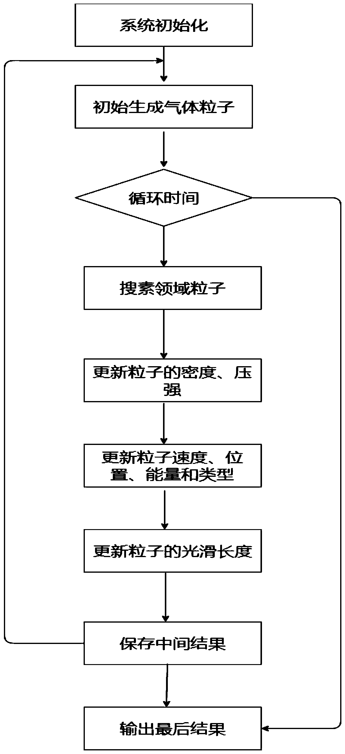
[0064] Step 1, initialization: related variables and particle information of the initialization system;
[0065] Step 2, generating particle information;
[0066] Step 3, list the solution equations and iteratively calculate:
[0067] According to the principle of the natural gas pipeline problem, the mathematical model of the physical model can be obtained, that is, the governing equation in the Lagrangian form is:
[0068]
[0069]
[0070]
[0071] wh...
PUM
 Abstract
Description
Claims
Application Information