Multi-mobile-robot formation method based on distributed preset time state observer
A technology of mobile robots and state observers, which is applied in the direction of instruments, motor vehicles, non-electric variable control, etc., can solve the problems of not being able to complete task requirements well, and achieve the effects of improving effects, high precision, and ensuring accuracy
- Summary
- Abstract
- Description
- Claims
- Application Information
AI Technical Summary
Problems solved by technology
Method used
Image

Examples
Embodiment Construction
[0045] In order to better understand the content of the patent of the present invention, the technical solution of the present invention will be further described below in conjunction with the drawings and specific embodiments.
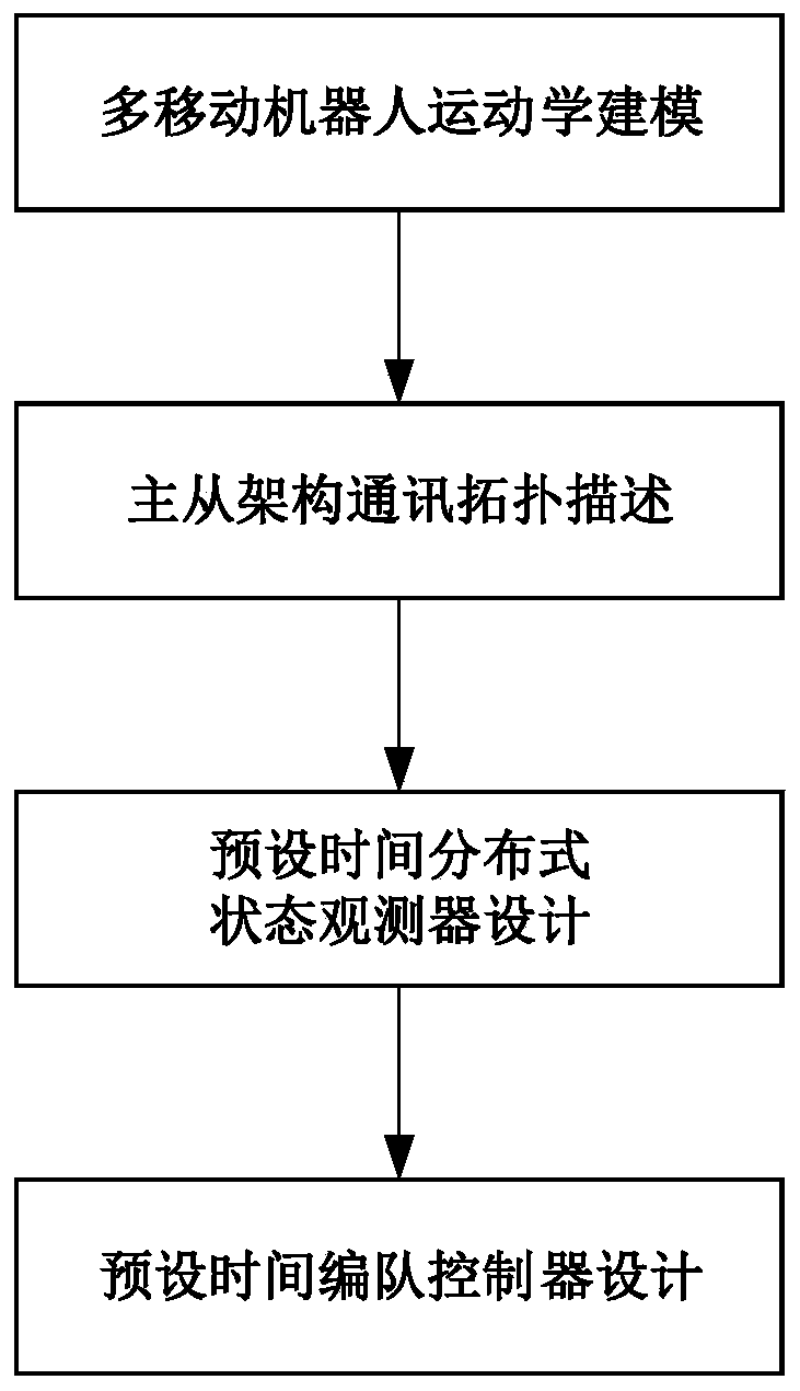
[0046] Such as Figure 1-6 As shown, the multi-mobile robot formation method based on the distributed preset time observer includes the following steps:
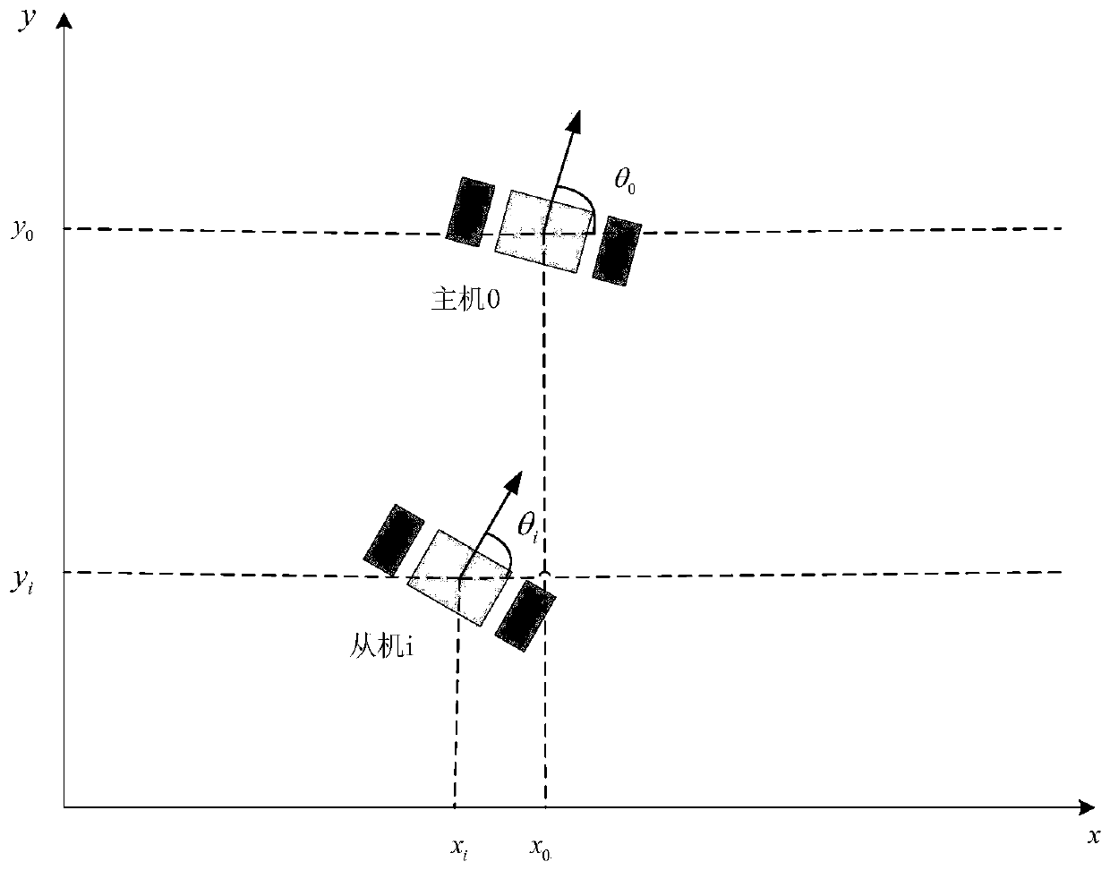
[0047] Step 1: Kinematics modeling: According to the operational characteristics of the multi-mobile robot, the kinematic equations of the multi-mobile robot are established, where the kinematic model of the multi-mobile robot is as follows figure 2 shown. The mobile robot is selected as a wheeled robot under the two-dimensional plane of the global coordinate system, and its kinematic equations can be described as follows:
[0048]
[0049] Among them, i is the number of mobile robot; N is a normal number, indicating the number of multiple mobile robots; Δ={1,2,...,N} is the number set of mult...
PUM
 Abstract
Description
Claims
Application Information
PatSnap Eureka turns technology decisions into work you can execute. Powered by our Innovation Knowledge Graph, it runs expert workflows across engineering, life sciences, materials and intellectual property. Get your review-ready output in minutes.


