Efficient multiscale finite element method for simulating two-dimensional water flow in porous media
A porous medium and finite element technology, applied in the field of hydraulics, can solve the problem of high consumption of basis function construction, achieve the effects of reduced calculation time, high element flexibility, and strong anti-deformation ability
- Summary
- Abstract
- Description
- Claims
- Application Information
AI Technical Summary
Problems solved by technology
Method used
Image
Examples
Embodiment 1
[0055] Example 1: Continuum model of two-dimensional steady flow
[0056] The research area is a square area: Ω=[50m, 150m]×[50m, 150m], permeability coefficient K(x,y)=x 2 m / d, the research equation is the steady flow equation:
[0057]
[0058] Boundary condition is constant head boundary condition The source-sink item is 0, and this model has an analytical solution: H=x 2 -3y 2 .
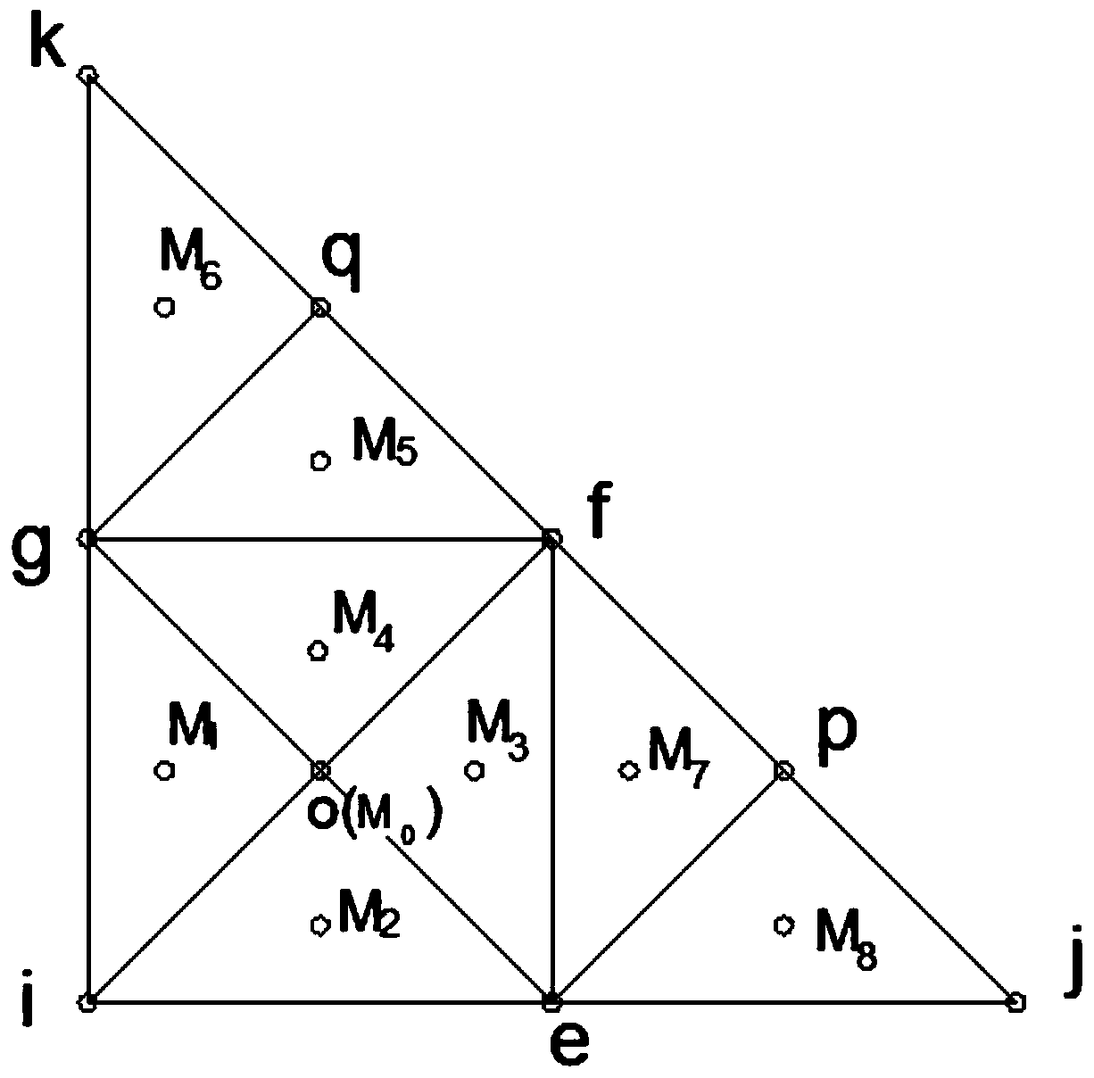
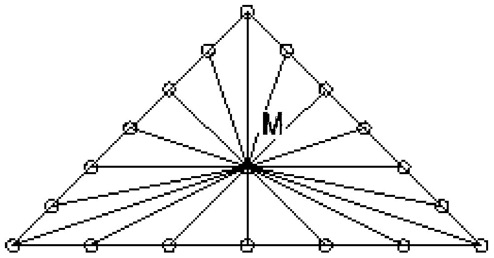
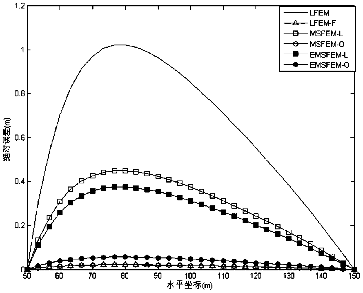
[0059] Sub-example 1.1: Solved using LFEM, LFEM-F, MSFEM-L, MSFEM-O, EMSFEM-L and EMSFEM-O. LFEM-F divides the study area into 88200 units, other methods divide the study area into 1800 units; MSFEM divides each coarse grid unit into 49 fine grid units (7×7), EMSFEM divides each A coarse grid is divided into 8 medium grid units, each medium grid unit is divided into 6 fine grid units, a total of 48 fine grid units.
[0060] image 3 is the absolute error value of the water head at the y=100m section of the above numerical method, it can be seen that the error of LFEM is the largest, th...
Embodiment 2
[0066] Example 2: Gradient medium model of two-dimensional unsteady flow
[0067] The research area is a square area: Ω=[0,10km]×[0m,10km], the research equation is:
[0068]
[0069] The thickness of the aquifer in the study area is 10m, and the left and right sides are the boundaries of constant water head, the water heads are 10m and 0m respectively, and the upper and lower sides are separated from each other. The permeability coefficient increases from 1m / d to 250m / d from the left boundary to the right boundary, that is, K(x,y)=1+x / 40m / d, and the water storage coefficient S=0.00001-0.000009x / 1000 / m, at coordinates ( There is a pumping well at 5200m, 5200m) with a flow rate of 1000m 3 / d. The water head at the initial moment changes linearly from left to right: H 0 (x, y) = 10-x / 1000m.
[0070] Sub-example 2.1: In this example, the pumping time is 5 days and the time step is 1 day. LFEM, LFEM-F, MSFEM-L, MSFEM-O, EMSFEM-L and EMSFEM-O are used to solve the problem. ...
Embodiment 3
[0078] Embodiment 3: two-dimensional submerged flow model (non-linear model)
[0079] The research equation is the Boussinesq equation:
[0080] -▽·K(x,y,H)▽H=W,
[0081] All parameters in this example have been dimensionless and have no units; the study area is: Ω=[0,1]×[0,1], the boundary water head is the boundary of constant head and both are 0, the base level b=-4, the permeability coefficient for:
[0082]
[0083] Where T=(1+x)(1+y), the initial water head is 0, this model has an analytical solution: H=xy(1-x)(1-y), and the source-sink term W is given according to the analytical solution.
[0084] The Boussinesq equation is a nonlinear equation that can be solved iteratively:
[0085] -▽·K(x,y,H (n-1) )▽H (n) =W,
[0086] The set iteration error is η=10 -4 , that is, iterate until |H (n) -H (n-1) |<η.
[0087] Using MSFEM-O and EMSFEM-O to solve this example, the study area is divided into 1800 parts. MSFEM divides the coarse grid unit into 49 fine grid un...
PUM
 Abstract
Description
Claims
Application Information