Method and apparatus for creating time-optimal commands for linear systems

Abstract

The system described herein determines an input command profile for a dynamic system that can be modeled as a linear system, the input command profile for transitioning an output of the dynamic system from one point to another point. The system identifies characteristics of the dynamic system, and then selects a command profile which defines an input to the dynamic system based on the identified characteristics. The command profile comprises one or more pulses which rise and fall at switch times, and the command profile is useable with substantially any dynamic system that can be modeled as a linear system. The system then imposes a plurality of constraints on the dynamic system, at least one of the constraints being defined in terms of the switch times, and determines the switch times for the input to the dynamic system based on the command profile and the plurality of constraints.

Description

1. Field of the InventionThe present invention is directed to a system for creating commands that increase the speed of system response. The invention can be applied to virtually any type of machine, process, or entity that can be modeled linearly. In particular, the invention deals with the creation of command profiles that are time-optimal, meaning commands that will move a system from one rest state to another rest state in the shortest amount of time. To this end, the invention provides a three-step procedure for generating time-optimal command profiles for all types of linear single-input, single-output systems. Constraint equations that result from this approach are both notationally and computationally simple. Consequently, the invention delivers results for complex systems faster and more reliably than traditional approaches. The invention furthermore incorporates additional practical constraints into its solution framework, thereby producing different types of time-efficien...

AI Technical Summary

Problems solved by technology

In some situations, however, this is not enough.

Many systems, however, do not tolerate these types of changes.

An engineer at a hydroelectric plant, for example, would be foolhardy to consider building a new dam to better control the power output.

Similarly, commissioning the Space Shuttle to install new sensors on an operating weather satellite might also prove equally absurd.

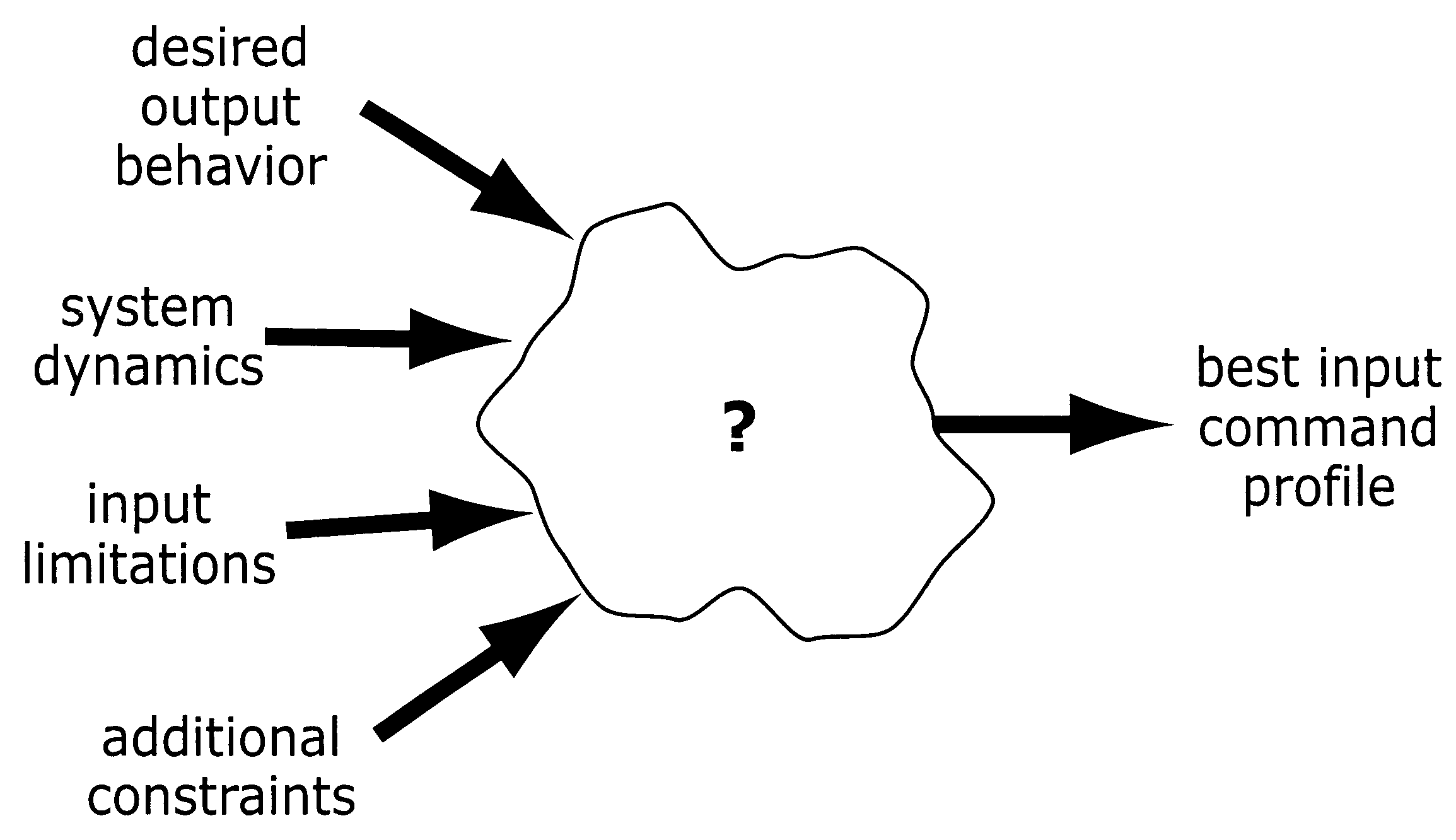
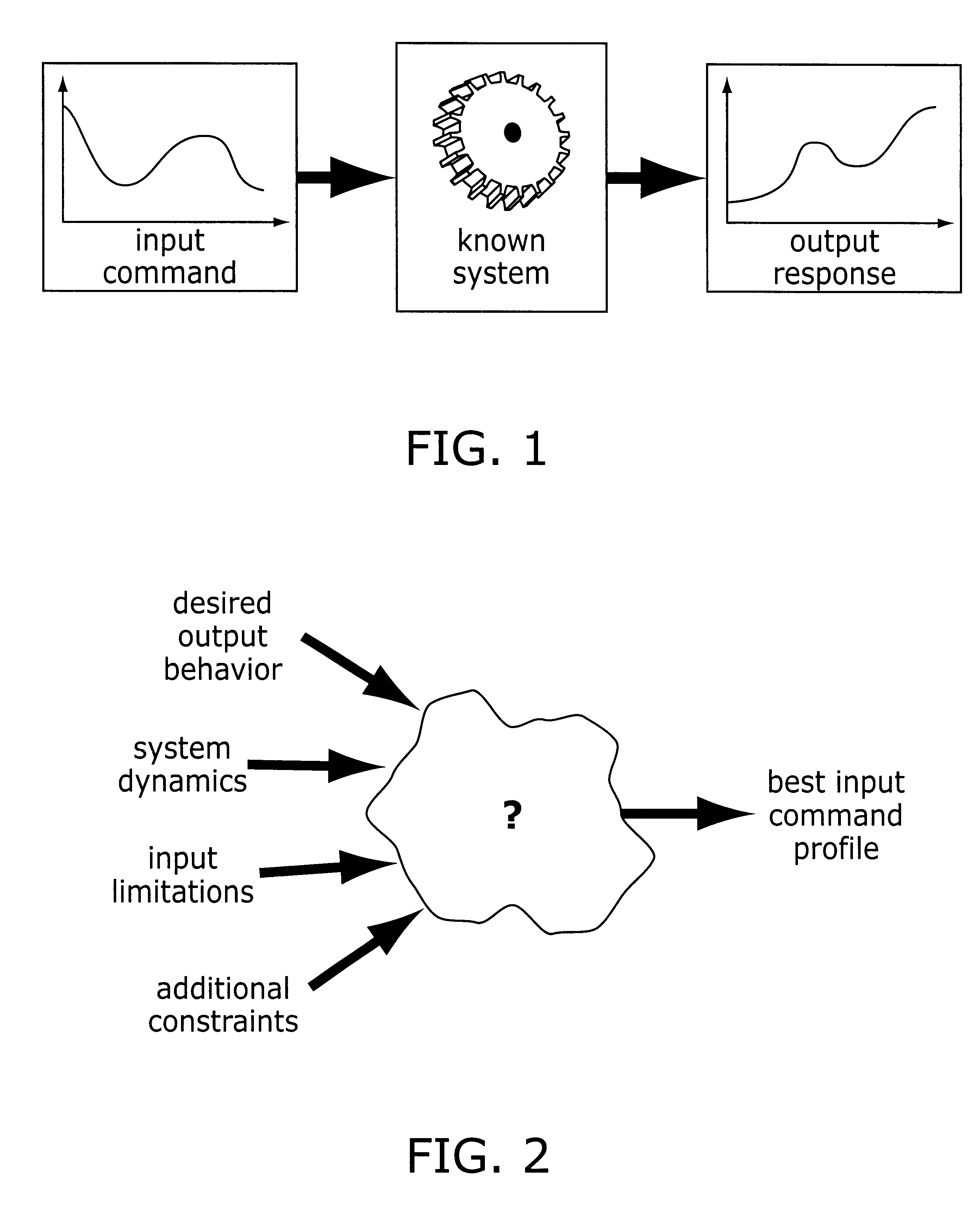
The problem facing designers who wish to improve the performance of their systems, which can be called "the feedforward control problem", addresses the question of how to select the input command for a given system that produces the most desirable output response.

As an unfortunate side-effect of these performance enhancements, undesirable machine dynamics often become the primary barrier to further performance improvements.

However, due to design limitations, actuator capacity must often be restricted.

In this regard, in addition to accounting for desired output behavior, system dynamics, and input limitations, many systems may be sensitive to other performance variables.

Other systems may have additional requirements such as limitations on internal loading or energy efficiency.

This problem statement, however, is far too general to lend insight into a solution approach.

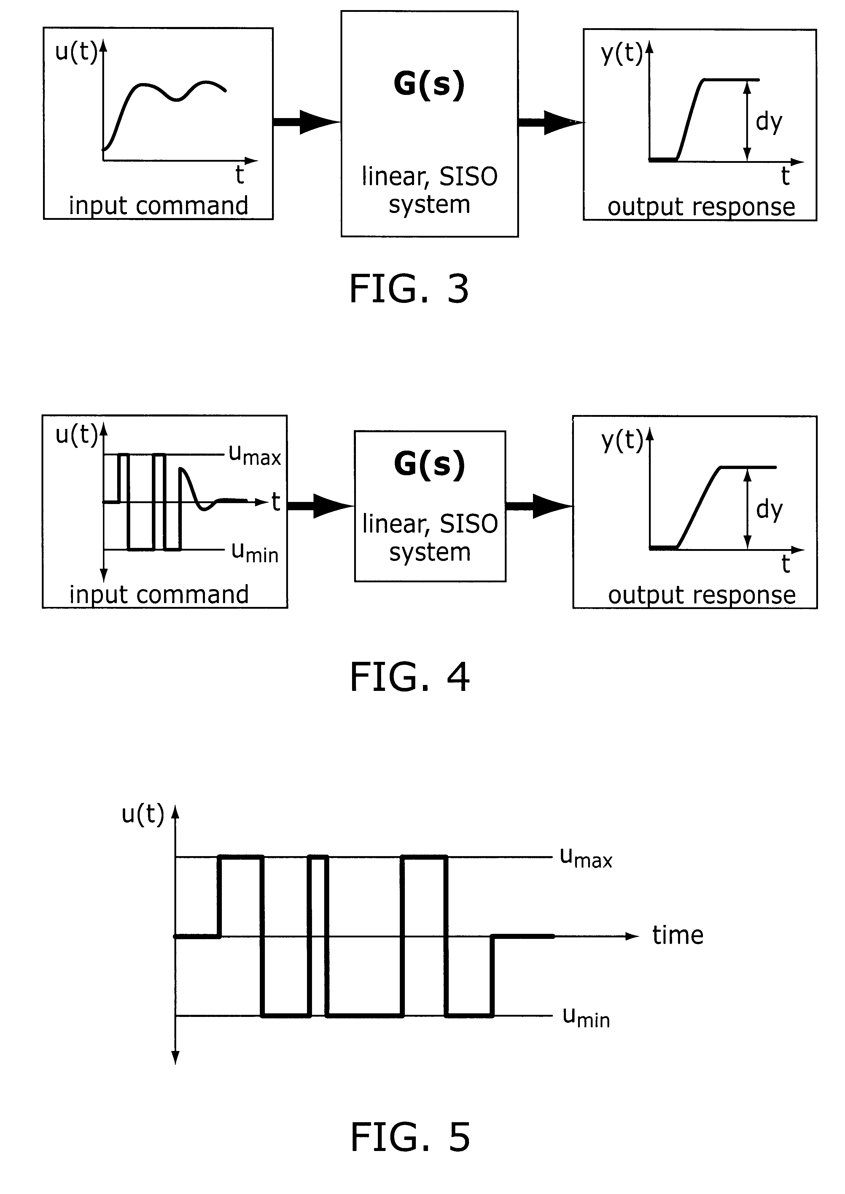
Third, it will be assumed that the goal of the problem is to transition the system output rapidly from one rest state to another rest state.

With this long history of research, it is difficult to know where to begin to describe the state of the art.

In approaching this task, design engineers typically face a variety of design tradeoffs that influence the construction of the hardware and the performance of the machine.

Primarily due to space, weight, and power constraints, this is not always possible.

When design considerations do not allow for this kind of hardware augmentation, the design engineer must turn to feedback approaches to eliminate undesirable system dynamic behavior.

However, in some systems, such as ones where sensor feedback is unavailable, high-performance control is not an option.

While closed-loop control techniques are used for minimizing error in the face of disturbances, they cannot always be optimized for the task at hand.

The time-optimal control problem, as stated above, is concerned with finding the fastest possible ways to move systems from one state to another.

Due in part to the complexity of these initial approaches and since energy-based control methods promised greener pastures, work in this area was largely abandoned.

Unfortunately, applying these tools to the task of deriving commands for a given system is not immediately straightforward.

A number of techniques have been proposed for doing this, but all are numerically intensive and largely too unreliable to be applied to a wide class of systems.

Although solution techniques are numerically complex and unreliable, many researchers have set these processes to the task of deriving time-optimal commands for nonlinear systems.

First, largely due to the complexity of numerical and iterative approaches for solving this problem, much of the recent work in this area has focused on making statements about the general nature of optimal commands in order to reduce the size of the solution space.

Research results revealed that, although input shaping is inherently a digital filtering technique, conventional digital filters, since they are not intended for mechanical systems, cannot equal the performance of input shapers.

Unfortunately, due the nature of the constraints in Pontryagin's principle, iterative search routines can be numerically intensive and solutions can be elusive.

Largely due to this inherent complexity, these types of solution approaches have seen limited application on complex systems.

What is yet unavailable, however, is a simple approach that can be applied with generality to virtually all types of linear systems.

As outlined above, the time-optimal control problem places a strict set of constraints on system response to a time-optimal command profile.

In general, finding a D(s) to exactly cancel G(s) is not often possible.

Additionally, since the equations are algebraic and implemented as vector operations, computational requirements are small.

For systems with repeated roots, the dynamics cancellation equations prove to be somewhat more complex to express.

Additionally since all of the calculations in this code are algebraic and can be expressed largely as vector operations, the computational requirements of this code are small.

The second boundary condition, which requires that the system output change by the desired amount, dy, is more complicated to express.

This numerically intensive procedure would likely result in undesirably long solution times.

Since this type of command will eventually exceed the system actuator limits, there is no time-optimal command that will satisfy the problem constraints.

However, it is difficult to derive a general analytic expression for the solution of equation 3.23 using this approach.

In these situations, the integral in equation 3.35 will not converge as t goes to .infin.. However, as will be discussed later herein, creating time-optimal commands with undamped or unstable oscillation is bad design practice and should not be implemented on a real system.

In order to implement this equation, all that is required is to take the limit of N(s)/D(s), which is trivial given the system transfer function, and to integrate u(t) from 0 to .infin. rbp times. To perform this integration, a numerical integration routine could be performed during the problem optimization, but this is very numerically intensive.

However in most cases, the

Images