[0034] The present invention will be further clarified below in conjunction with specific examples. It should be understood that these examples are only used to illustrate the present invention and not to limit the scope of the present invention. After reading the present invention, those skilled in the art will understand various equivalent forms of the present invention. All modifications fall within the scope defined by the appended claims of this application.
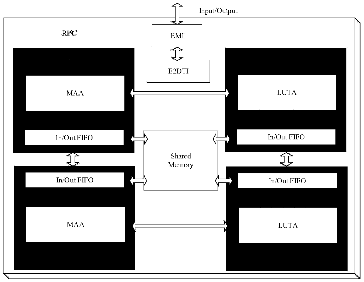
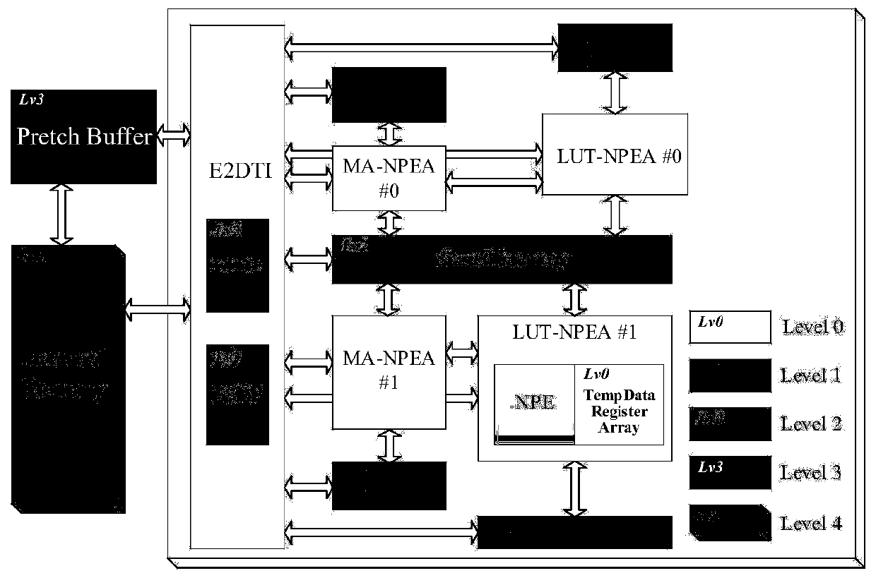
[0035] Such as figure 1 As shown, the computing array of the Convolutional Neuron Processing Unit (CNPU) adopts a heterogeneous design. The CNPU calculation subsystem includes a calculation array MA-NPEA based on a multiply-add circuit, a calculation array LUT-NPEA based on a look-up table multiplier, and a shared memory between arrays (Shared Memory). Two for each calculation array. MA-NPEA is composed of basic circuits such as approximate multipliers and approximate adders, and is suitable for convolutional layers with large computational tasks and large weighted bit widths. LUT-NPEA is mainly composed of a look-up table based on one-write-multiple-read SRAM and an arithmetic logic unit, which is suitable for convolutional layers with small weighted bit width and a large number of repeated multiplication calculations. The convolution processing unit flexibly allocates computing arrays according to the characteristics of each network layer and task priority. Array expansion includes heterogeneous array expansion and homogeneous array expansion.
[0036] For the convolution calculation tasks of large-size feature maps or convolution kernels, although cutting can be done, image cutting will cause data redundancy, waste storage resources, and increase memory access bandwidth requirements. In order to maximize the data reuse rate and computing performance, and save storage resources, CNPU can splice the same type of NPEA arrays to achieve the expansion of homogeneous arrays, which can increase the size of image blocks and reduce storage resources and bandwidth. Occupy, improve computing performance and meet task requirements.
[0037] For convolutional layers with a large number of repeated multiplication operations, schedule LUT-NPEA to implement multiplication operations based on lookup tables. Since LUT-NPEA uses lookup tables to achieve multiplication calculations, lookup table data updates rely on MA-NPEA in the preprocessing stage Realized by the computing unit. In order to reduce the data transmission delay between the arrays, a one-way data transmission path is added between MA-NPEA#0 and LUT-NPEA#0 and between MA-NPEA#1 and LUT-NPEA#1. Through this data transmission channel, heterogeneous array expansion can be realized. Through pipeline operation, the cooperative work of various heterogeneous arrays can be realized.
[0038] In application scenarios with extremely high performance requirements, CNPU allows four arrays to run at the same time to achieve full expansion of the array and maximize the utilization of computing resources.
[0039] Such as figure 2 As shown, when interacting with external memory, data storage is optimized by grading the storage architecture of the memory. Level 0 is the internal temporary data register of the computing unit. The temporary data register (Temp DataRegister) is tightly coupled with the neuron processing unit NPE, and each computing unit NPE has a corresponding temporary register for temporarily storing intermediate results. Level 1 is a distributed data cache closely coupled to the computing array, and Level 2 is a data cache between the accelerator and external storage. Level 3 is the prefetch cache. Level 4 external storage.
[0040] Such as image 3 As shown, the data transmission between the convolution processing unit CNPU and the external memory is realized through the external memory access interface EMI. Since convolutional network calculations need to read a large amount of two-dimensional data, traditional EMI is not suitable for accessing two-dimensional data, and a large part of the read data will be wasted. Therefore, the external 2D Data Transfer Interface (E2DTI) customized in this article can convert and transmit 2D data such as feature maps and convolution kernel data. E2DTI converts the CNPU's 16-bit feature map data request and the mixed bit width weight data request into a 64-bit data request. The external two-dimensional data conversion interface E2DTI is mainly composed of three independent modules: data transmission control module, data reading module and data writing back module. After the data read module (Data Read, DR) sends the data access request to the EMI, the returned data is sent to the ELDF. The Data Write (DW) module temporarily stores the data from the convolution processing unit into the ESDF. When the data in the ESDF accumulates to a certain amount, it is written to the corresponding location in the external storage at one time through EMI. When DR and DW access EMI at the same time, the data transmission control module DTC can decide which module to authorize external memory access rights. In order to ensure the consistency of data, the data transfer control module (Data Transfer Control, DTC) prioritizes the authorization of external memory access to DW.
[0041] When reading data from external memory, the external two-dimensional data conversion interface E2DTI converts the read data access request of multiple bit widths of the convolution processing unit CNPU into an external memory access request in units of 64 bits and sends it to EMI. EMI reads the required data from the external memory according to the data request and transmits it to E2DTI. E2DTI splits the data returned by EMI and transfers the data to the distributed storage unit DM. When writing data to external storage, the external two-dimensional data conversion interface E2DTI still first converts the data access request of the convolution processing unit CNPU into a write data request in units of 64 bits, and then sends the write request to EMI. At the same time, E2DTI splices the data to be written back to external storage. The external storage access interface EMI writes data to the corresponding location of the external storage according to the write request.
[0042] The data scheduling of MA-NPEA is shown in Figure 4. If MA-NPEA has k rows of computing units, then the distributed storage DM has k+1 banks. Taking k equal to 8 as an example, the data scheduling of MA-NPEA is shown in Figure 4. An arc of the outer ring represents a row of MA-NPEA calculation units, a total of 8 rows of calculation units. The inner arc represents the bank of distributed storage (DM), and distributed storage contains 9 banks. The distributed storage and computing array adopts a fully connected flexible routing interconnection structure, and each bank can provide computing data for any row of computing units in the MA-NPEA computing array. As shown in Figure 4(a), the first to eighth banks of distributed storage are preloaded with the first eight rows of data of the feature map. In the first operating cycle, the data of the first to eighth banks are sent to MA-NPEA for calculation. At this time, the i-th Bank is mapped to the i-th row calculation unit of MA-NPEA one by one. While the MA-NPEA array is calculated, the 9th Bank begins to preload the 9th row of input data. As shown in Figure 4(b), after completing the calculation of the first cycle, the convolution kernel moves down one line to start a new convolution operation. The inner ring rotates counterclockwise by one unit, indicating that distributed storage and MA- The row calculation unit of NPEA generates a new mapping relationship. At this time, the i+1th Bank provides input data for the i-th row calculation unit. The calculation array no longer uses the data of the first bank. Therefore, the data of the first bank is invalid and no longer provides data for the array. The data pre-loaded in the ninth bank in the previous cycle can be used in the calculation of the eighth row of the calculation unit in this cycle. In the second operating cycle, when MA-NPEA is calculating, the first bank begins to preload the 10th row of data. As shown in Figure 4(c), when the calculation is completed in the second operating cycle, the inner ring continues to rotate counterclockwise by one unit, and the distributed storage and computing array start a new interconnection and enter the third operating cycle. In the third operating cycle, the second bank is free for pre-loading the 11th row of data, and the first bank provides data for the 8th row of the calculation unit. Repeat the above process until the convolution operation is completed. Every time a cycle of computing tasks is completed, the distributed storage must rotate a unit counterclockwise to perform a new mapping with the computing array. Most of the bank data in the distributed storage DM can continue to be used by computing units in other rows. Every time a new operating cycle is entered, a bank is always free for prefetching data, and at the same time, a bank is always added to the array calculation. This kind of distributed storage with flexible routing structure fully realizes data reuse. Except for the first bank in the first cycle, the data in each bank can be reused multiple times, realizing data reuse between rows of convolution operations. Data reuse is realized through distributed caching and flexible routing, avoiding repeated data acquisition from external storage, and reducing memory access power consumption.
[0043] The LUT-NPEA calculation array inherits two working modes of the look-up table multiplier: Figure 5 The multiplication split mode shown and as Image 6 The product query mode shown.
[0044] In the multiplication and splitting working mode, in order to make full use of the lookup table resources, combined with the parallelism of the convolution algorithm, the effective utilization of the lookup table is improved by serializing the feature map data. The feature map serialization scheduling method is based on the convolution parallel computing strategy with the feature map changing and the convolution kernel fixed. Such as Figure 5 As shown, there are a total of n feature maps in the figure, and each pixel is represented by a two-digit index. The first number represents the number of the feature map, and the second number represents the index of the pixel in this feature map. Through the convolutional network compression strategy in this article, multiple feature maps can share a two-dimensional convolution kernel. For example, the first pixel of each feature map in the figure is multiplied by the first weight w1 of the convolution kernel, and the result is stored in the first lookup table. The first lookup table needs to be queried at least n times. In fact, the average number of reuses of each lookup table is much greater than n.
[0045] Such as Figure 5 As shown, the elements at the corresponding positions of the n feature maps are arranged into one-dimensional data, stored in the address FIFO of the look-up table, and then sent to the look-up table in order of first-in first-out, and the convolution weight and the corresponding pixel are obtained The product of the data. Considering the reusability of the feature map data, a flexible routing structure is adopted to connect the output port of each address FIFO to the input port of other FIFOs to realize the data reuse of the feature map. When the step size is 1, the output of each FIFO is connected to the input port of the adjacent FIFO on the left, such as Figure 5 Shown by the solid line. When the step size is 2, the output of each FIFO is connected to the input port of the FIFO with a look-up table address interval, such as Figure 5 Shown by the dotted line. The routing relationship between the address FIFOs is configured according to the step length of the convolution kernel movement.
[0046] In the product query mode, the parallel access rate of the lookup table is improved by serializing the convolution kernel data. The convolution kernel serialization scheduling needs to cooperate with the convolution parallel computing strategy that the feature map is unchanged and the convolution kernel is changed. Assuming that the weight of the convolution kernel is quantized by 4 bits, there are 16 possibilities. In the product query mode, the lookup table stores the result of the product of the input data and the 16 weights. Similar to the multiplication split mode, the same feature map can be convolved with n convolution kernels. Such as Image 6 As shown, the first element of the feature map can be multiplied by the first weight of each convolution kernel. Therefore, the weights of the corresponding positions of n convolution kernels can be combined into one-dimensional data and sent to the lookup table. Address FIFO. Unlike the multiplication split mode, the feature map data in this mode cannot be reused. However, because the convolution kernel data is reused, each address FIFO is connected end to end to realize the repeated recycling of the convolution kernel.