Compressed sensing-based antifriction bearing fault diagnosis method under working condition disturbance condition
A technology of fault diagnosis and compressed sensing, which is applied in mechanical bearing testing, computer components, instruments, etc., can solve problems such as difficult bearing fault diagnosis, difficult small sample fault detection, and changes in the working environment, so as to reduce the consumption of computing resources and The effect of bandwidth consumption, reduced amount of sampled data, and short runtime
- Summary
- Abstract
- Description
- Claims
- Application Information
AI Technical Summary
Problems solved by technology
Method used
Image
Examples
Embodiment
[0110] In order to compare this embodiment with other fault diagnosis algorithms, the present invention uses the open rolling bearing data of Case Western Reserve University in the United States for fault diagnosis to show the effectiveness of the algorithm of the present invention.
[0111] The test bench includes a 2HP motor, a torque sensor, a power meter and a set of control circuits. The single-point fault in the test was machined by EDM with a fault diameter of 0.533 mm. The data is collected using an accelerometer mounted on a magnetic base, specifically at the end at 12 o'clock. The digital signal is obtained through discrete sampling, and its sampling rate is 12K / s.
[0112] The data used in the present invention is as shown, and the data length is 56000.
[0113] Table 1 Data Details
[0114]
example 1
[0115] Example 1: Example of Bearing Fault Diagnosis under Condition Disturbance
[0116] The concrete steps of this embodiment are as follows:
[0117] Step 1. Construction and compression of the reference matrix.
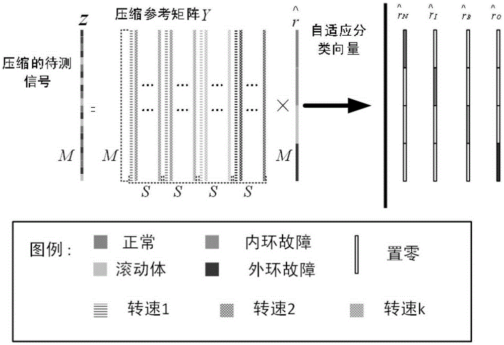
[0118] In this example, N is set for each failure mode t =56000,N=800,N t / N=70, using 50 data segments as reference samples and 20 data segments as test samples. Therefore b ORM =b CRM =50, b Test =20, so the size of the orthogonal reference matrix is 800×(50*4*4), such as Figure 5 (A) shown. In the figure, the Y axis represents the length of each signal segment, and the X axis represents each signal segment. The structure of the orthogonal reference matrix is shown in Table 2.
[0119] Table 2 Orthogonal reference matrix structure
[0120]
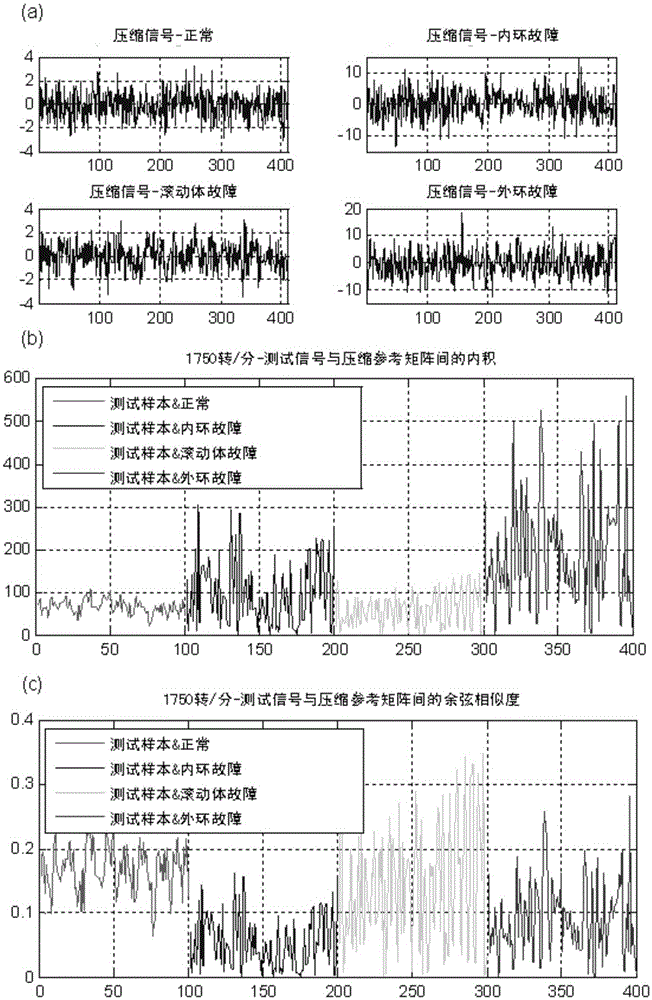
[0121] In this example, a Gaussian random matrix is used as the measurement matrix, the compression rate is set to 0.5, and the length of the original signal is 800, so the length of the compressed signal ...
example 2
[0132] Example 2: Example of Vibration Signal Reconstruction
[0133] Considering that the effectiveness of vibration signal reconstruction has nothing to do with the rotational speed, the sampling rate of the vibration signal in this example is 12,000 per second, and the rotational speed is 1750 rpm. In this example, the compressed signal in Example 1 is used to verify the effectiveness of the reconstruction.
[0134] In this example, the length of the original signal segment is N=800, the length of the compressed signal segment is M=400, the compression ratio CR=M / N=0.5, and the number of signal segments b=50.
[0135] The orthogonal basis matrix used in this example is the Fast Fourier Transform matrix, such as Figure 11 As shown, its size is 800×800.
[0136] Reconstruction of sparse vectors using measurement matrices, orthonormal basis matrices, and compressed signals by matching pursuit algorithm ( The size is 800x1). Unlike fault diagnosis, the number of iterati...
PUM
 Abstract
Description
Claims
Application Information


