[0023] The technical solutions of the present invention will be described in detail below one by one, and the purpose and effect of the present invention will be more obvious.
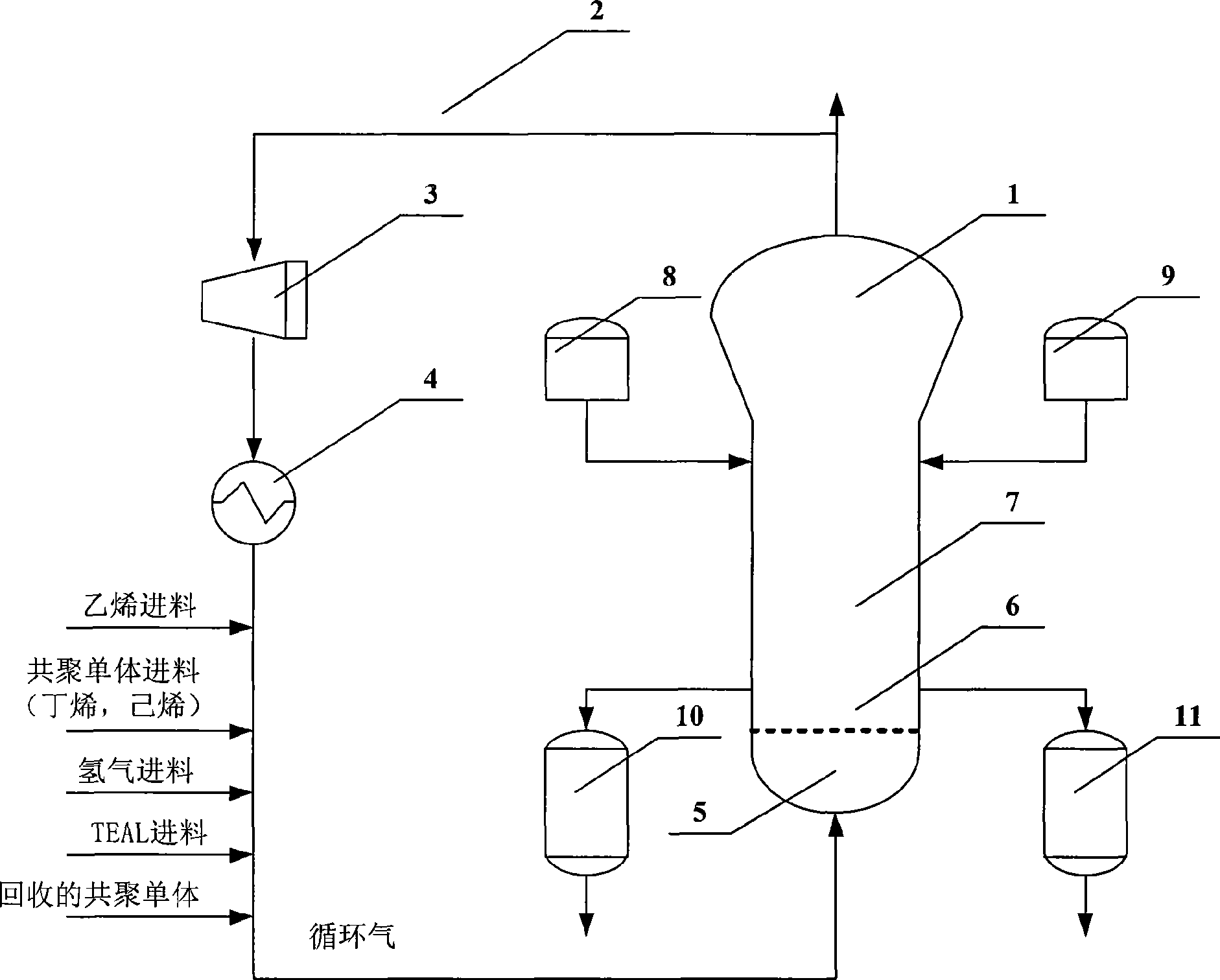
[0024] figure 1 It is a schematic diagram of a common industrial fluidized bed gas-phase polyethylene production device in China. The main equipment is composed of a gas-phase fluidized bed reactor 1, a circulating gas pipeline 2, a circulating gas compressor 3, and a circulating gas heat exchanger 4. The circulating gas pipeline is connected in series. Among them, the gas-phase fluidized bed reactor includes a reactor mixing chamber 5, a reactor distribution plate 6, a fluidized bed layer 7, a product discharge tank A 8, a product discharge tank B 9, a catalyst feeder A 10, a catalyst feeder B11 is attached to the inside and outside of the reactor. During the production process, the circulating gas containing monomers, comonomers and other components first enters the mixing chamber 5 at the bottom of the reactor, and then enters the fluidized bed 7 through the specially designed reactor distribution plate 6 after premixing. While the polymer/catalyst powder is suspended and fluidized for polymerization reaction, the polymerization heat is transferred to the fluidizing gas and taken out of the reactor. The higher temperature gas leaving the reactor is recirculated into the reactor at a lower temperature after being compressed, heat exchanged and supplemented with raw materials. The catalyst required for the reaction process is fed into the reactor through the catalyst feeder A 10 or/and the catalyst feeder B 11. The polymer product is discharged alternately in batches through discharge tank A 8 and discharge tank B 9 to keep the height of the fluidized bed constant. In this way, the continuous operation of the production process is realized.
[0025] The soft measurement method of the product quality of the industrial fluidized bed gas-phase polyethylene device of the present invention includes the following steps:
[0026] (1) Select 29 field measurement variables that have a direct impact on the quality of polyethylene resin as auxiliary variables of the soft measurement model to form the measurement parameter vector X m.
[0027] The 29 selected on-site measurement auxiliary variables are: reactor inlet temperature T_Rxinlet, reactor temperature T_RX, reactor outlet temperature T_RXoutlet, ethylene feed temperature T_Ethylene, butene feed temperature T_Butene, reactor pressure P_Reactor, ethylene feed pressure P_Ethylene, product discharge tank A pressure drop P_TankA, product discharge tank B pressure drop P_TankB, reactor distribution plate pressure drop P_RXplate, circulating gas flow F_Cyclegas, ethylene feed flow F_C2H4, butene feed flow F_C4H8, hydrogen feed flow F_H2, nitrogen feed flow rate F_N2, triethylaluminum injection rate F_TEAL, reactor productivity F_Prorate, hydrogen/ethylene mol ratio R_H2toC2, butene/ethylene mol ratio R_C4toC2, catalyst feeder A speed V_FeederA, catalyst feeder B speed V_FeederB , Reactor bed weight W_Bed, reactor level indicator value L_Bed, reactor upper bulk density D_Upper, reactor lower bulk density D_Lower, ethylene concentration in circulating gas M_C2H4, butene concentration in circulating gas M_C4H8, hydrogen concentration in circulating gas M_H2 , The nitrogen concentration in the circulating gas is M_N2. The combined measurement parameter vector X m Is: X m =[T_Rxinlet T_RX T_Rxoutlet T_Ethylene T_Butene P_ReactorP_Ethylene P_TankA P_TankB P_Rxplate F_Cyclegas F_C2H4 F_C4H8 F_H2 F_N2F_TEAL F_Prorate R_HedtoC2 V_C4 L_Feed_Low_Ber2 M_Hed_Ber2 M_C4 L_Feed_Ber2 M_C4 D_HedtoC2 V_C4
[0028] (2) Select two variables that characterize the quality level of polyethylene resin as the soft measurement target variables to form the soft measurement parameter vector Y m.
[0029] The two selected soft measurement target variables are: resin melt index MI and resin density ρ. The combined soft-sensing parameter vector Ym Is: Y m =[MI ρ].
[0030] (3) Collect a set of soft-sensing modeling sample sets during the normal operation of the gas-phase fluidized bed device i=1, 2...NN, constituting the modeling sample matrix XX and YY.
[0031] Modeling sample set i=1, 2...NN, the modeling sample matrix formed is:
[0032] XX = [ X m 1 X m 2 · · · · · · X m NN ] T
[0033] YY = [ Y m 1 Y m 2 · · · · · · Y m NN ] T ;
[0034] among them, Is the measurement parameter vector X m The sample value of the i-th sample point, Is the soft sensor parameter vector Y m The sample value of the i-th sample point, NN is the number of sample points in the modeling sample set, and its value is between 1000 and 1200.
[0035] (4) Standardize and normalize the modeling sample matrix XX and YY (make the mean value of each variable 0 and variance 1) to obtain the normalized modeling sample matrix X 0 And Y 0.
[0036] When standardizing and normalizing the modeling sample matrix XX and YY, the specific formula used is:
[0037] Mean calculation: XX ‾ = 1 NN Σ i = 1 NN XX i , YY ‾ = 1 NN Σ i = 1 NN YY i ,
[0038] Variance calculation: σ XX 2 = 1 NN - 1 Σ i = 1 NN ( XX i - XX ‾ ) , σ YY 2 = 1 NN - 1 Σ i = 1 NN ( YY i - YY ‾ )
[0039] Normalized calculation: XX 1 = XX - XX ‾ σ XX , YY 1 = YY - YY ‾ σ YY ;
[0040] Where, XX, YY, They are the mean and variance corresponding to XX and YY, respectively. Divide the sampling data of the NN sample points in the modeling sample matrix into a training sample matrix and a test sample matrix according to the proportion, and then obtain the input matrix X of XX and YY composed of the training sample matrix 0 And output matrix Y 0 , X 0 Each row of is an input vector, Y 0 Each row of is an output vector.
[0041] (5) According to X 0 And Y 0 , To establish a non-linear partial least square soft-sensing model for the product quality of an industrial fluidized bed gas-phase polyethylene device offline: X 0 = t 1 p 1 T + t 2 p 2 T + · · · · · · + t l p l T , Y ^ 0 = V 1 β 1 T + V 2 β 2 T + · · · · · · + V l β l T , Where t i , P i , I=1, 2,...l is X 0 The l principal component score vector and load vector obtained after principal component decomposition, β i , I=1, 2,...l is Y 0 About nonlinear expansion terms V i = 1 t i t i 2 , Class load matrix of i=1,2,...l. From P=[p 1 p 2 ……P l ], β=[β 1 β 2 ……Β 1 The two-tuple (P, β) formed by] is the parameter set of the soft sensor model.
[0042] Non-linear partial least squares soft sensor model X 0 = t 1 p 1 T + t 2 p 2 T + · · · · · · + t l p l T , Y ^ 0 = V 1 β 1 T + V 2 β 2 T + · · · · · · + V l β l T , It is realized by embedding Taylor series approximation on the basis of linear least squares model. Theoretically, the order of Taylor series approximation can be as high as any order. In general, the method of the present invention preferably uses a parabolic approximation (second-order) model. The soft-sensing model parameter set (P, β) is obtained through a cyclic recursive algorithm called NPLS, and the cross-check technique is used to determine the optimal number of principal elements l.
[0043] The adopted NPLS loop recursive algorithm consists of the following steps: (1) Standardize the measurement data matrix X and Y to X 0 , Y 0. Let u take Y 0 A column of (usually the column with the largest variance), calculate the weight vector w T = U T X 0 /u T u, and normalize ‖w‖=1; calculate pivot t=X 0 w/w T w; (2) Use linear least squares regression algorithm to estimate the principal variable polynomial coefficient α 0 , Α 1 , Α 2 , U=α 0 1+α 1 t+α 2 t 2 +h, and make s = u ^ , By s and Y 0 Calculate q T =s T Y 0 /s T s, normalized ‖q‖=1; (3) Recalculate u=Y 0 q/q T q; (4) Use the Newton-Raphson algorithm for u=α 0 1+α 1 (X 0 w)+α 2 (X 0 w) 2 +h recalculate the weight w, and normalize ‖w‖=1; (5) t=X 0 w/w T w, check the convergence of t; (6) If t does not converge and the number of loop iteration steps does not exceed the limit, go to (2), otherwise continue to (7); (7) Calculate s, q, u and α according to the latest t 0 , Α 1 , Α 2; (8) Calculate the pivot direction p T = T T X 0 /t T t; (9) Construct the residual matrix X 1 =X 0 -tp T , Y 1 =Y 0 -sq T; (10) Use X 1 , Y 1 Continue with the principal component decomposition and model calculation of the next model dimension until the required number of principal components is reached.
[0044] (6) During online operation and implementation, every time a new auxiliary variable measurement value is obtained, the current field measurement data matrix is substituted into the soft measurement model for prediction calculation, and the prediction result Carry out inverse normalization and inverse normalization to obtain the product quality target variable prediction data matrix or vector in the sense of the engineering unit.
[0045] The prediction result calculated by the soft sensor model When performing denormalization and denormalization, the specific formula used is:
[0046] YY ^ = σ YY * Y ^ + YY ‾
[0047] Where, YY, Is the mean and variance of the previous normalization and normalization.
[0048] (7) In order to ensure the accuracy of soft measurement during long-term operation, the soft measurement model parameter set (P, β) is automatically calibrated regularly (24 hours or 48 hours).
[0049] The correction formula used is:
[0050] P k + 1 = P k + λ P * 1 J ( Y k - Y ^ k ) T H P ( Y k - Y ^ k ) * Σ j = 1 J ( y k j - y k j ^ ) Σ j = 1 J | y k j - y k j ^ |
[0051] β k + 1 = β k + λ β * 1 J ( Y k - Y ^ k ) T H β ( Y k - Y ^ k ) * Σ j = 1 J ( y k j - y k j ^ ) Σ j = 1 J | y k j - y k j ^ |
[0052] Where (P k+1 , Β k+1 ) Is the value of the model parameter set in the next operating cycle (k+1 time), (P k , Β k ) The value of the model parameter set in this running cycle (the kth time), Y k with Respectively, the resin melt index MI and resin density ρ are a data vector composed of a total of J laboratory analysis values and corresponding soft-sensing predicted values in this operating cycle. The internal elements are the single-point analysis values. And single point soft measurement value Y k = [ y k 1 y k 2 · · · · · · y k J ] , Y k ^ = [ y k 1 ^ y k 2 ^ · · · · · · y k J ^ ] ; λ P And λ β Is the scale correction factor; H P And H β Forgetting factor weighting matrix corrected for soft sensor model parameter set. In the soft-sensing model automatic correction formula, the scale correction factor is between 0 and 1.0; the number of rows and columns of the forgetting factor weighting matrix are both Y in this running cycle k with The number of measured value points, the internal element values are all between 0 and 1.0.
[0053] The following describes the specific implementation of the present invention in detail through a typical implementation case in conjunction with the accompanying drawings.
[0054] 1 Process variables and quality variables of industrial fluidized bed gas-phase polyethylene production equipment
[0055] Take a Unipol process fluidized bed gas-phase polyethylene production device as an example. In order to achieve continuous production of the device, a computer distributed control system (DCS) is usually used to control and operate the operation of the equipment. The main process variables and quality variables are shown in Table 1. Shown.
[0056] Table 1: The main process variables and quality variables of the fluidized bed ethylene gas phase polymerization process
[0057] Serial number
[0058] 2 Hardware system architecture and network connection in implementation
[0059] The hardware system integrated for on-site implementation of applications is realized by relying on the three-tier system structure of Internet network connection, such as figure 2 As shown, the lower layer is the data interface machine 14 for data exchange with the main control DCS device 13 of the gas-phase fluidized bed polyethylene device 12 in the present invention, which is connected to the DCS device through a DCS data cable. The middle layer is a high-performance network server 15 that meets explosion-proof and dust-proof standards, such as HP servers, Dell servers, etc., and the soft-sensing model calculation and parameter set automatic correction of the present invention are realized on this layer. The upper layer is the monitoring workstation 16. In this method, all human-computer interaction operations and information display are implemented in these monitoring workstations.
[0060] 3 Implementation steps and technical content
[0061] Step 1: Online collection of operation data of gas-phase fluidized bed polyethylene plant
[0062] Select 29 production measurement auxiliary variables and 2 soft measurement variables, respectively:
[0063] X m=[T_Rxinlet T_RX T_Rxoutlet T_Ethylene T_Butene P_ReactorP Ethylene P_TankA P_TankB P_Rxplate F_Cyclegas F_C2H4 F_C4H8 F_H2 F_N2F_TEAL F_Prorate R_H2toC2 V_C4 D_Heder2 M_C4 D_Heder_B_Up
[0064] Y m =[MI ρ]
[0065] Generally, the normal operation data of each grade of polyethylene resin needs to be continuous for more than 48 hours (database collection period can be set from 10 to 30 seconds, the same below) and stored in the database; switching operation data of different grades of resin requires at least one complete switch The cycle is saved in the database; the operation data of the process start-up process (lasting for more than 24 hours) is saved in the database; the normal process running data of the process (lasting more than 20 hours) is saved in the database.
[0066] Step 2: From the modeling sample set i=1, 2...NN constitutes the modeling sample matrix:
[0067] XX = [ X m 1 X m 2 · · · · · · X m NN ] T
[0068] YY = [ Y m 1 Y m 2 · · · · · · Y m NN ] T ;
[0069] Among them, the number of sample points is 1000.
[0070] Step 3: Standardize and normalize the modeling sample matrices XX and YY to obtain a normalized modeling sample matrix X 0 And Y 0 , The specific formula used is:
[0071] Mean calculation: XX ‾ = 1 NN Σ i = 1 NN XX i , YY ‾ = 1 NN Σ i = 1 NN YY i
[0072] Variance calculation: σ XX 2 = 1 NN - 1 Σ i = 1 NN ( XX i - XX ‾ ) , σ YY 2 = 1 NN - 1 Σ i = 1 NN ( YY i - YY ‾ )
[0073] Normalized calculation: XX 1 = XX - XX ‾ σ XX , YY 1 = YY - YY ‾ σ YY
[0074] Step 4: Establish a soft-sensing model of nonlinear partial least squares of resin properties.
[0075] According to X 0 And Y 0 , To establish a non-linear partial least square soft sensor model for the product quality of an industrial fluidized bed gas-phase polyethylene plant X 0 = t 1 p 1 T + t 2 p 2 T + · · · · · · + t l p l T , Y ^ 0 = V 1 β 1 T + V 2 β 2 T + · · · · · · + V l β l T , P=[p 1 p 2 ……P l ], β=[β 1 β 2 ……Β 1 ], among them, the optimal number of principal elements l is determined by cross-checking, which is 6 in this case, and the soft sensor model parameter set (P, β) is calculated by the NPLS cyclic recursive algorithm.
[0076] Step 5: In the case of online operation, every time a new auxiliary variable measurement value is obtained, the current field measurement data matrix is substituted into the soft measurement model X 0 = t 1 p 1 T + t 2 p 2 T + · · · · · · + t l p l T , Y ^ 0 = V 1 β 1 T + V 2 β 2 T + · · · · · · + V l β l T Carry out forecast calculations and put the forecast results by YY ^ = σ YY * Y ^ + YY ‾ Perform denormalization and denormalization processing. In this implementation case, the maximum relative error between the predicted value of the model and the measured value is less than 3%, which meets the accuracy requirements of industrial applications.
[0077] Step 6: Automatic correction of soft-sensing model parameters, the correction algorithm is
[0078] P k + 1 = P k + λ P * 1 J ( Y k - Y ^ k ) T H P ( Y k - Y ^ k ) * Σ j = 1 J ( y k j - y k j ^ ) Σ j = 1 J | y k j - y k j ^ |
[0079] β k + 1 = β k + λ β * 1 J ( Y k - Y ^ k ) T H β ( Y k - Y ^ k ) * Σ j = 1 J ( y k j - y k j ^ ) Σ j = 1 J | y k j - y k j ^ |
[0080] In this implementation case, the correction formula parameter is set as: scale correction factor λ P And λ β Take the values 0.573 and 0.428 respectively, J is 24, and the forgetting factor weighting matrix H P And H β Both are identity matrices (weighted by equal forgetting factors).
[0081] The above is a specific and complete implementation process of the present invention, and this example is used to explain the usage of the present invention instead of limiting the present invention. Any changes made within the protection scope of the claims of the present invention belong to the protection scope of the present invention.