[0065] The present invention will be described in further detail below in conjunction with specific embodiments and with reference to the accompanying drawings.
[0066] The present invention provides a wheat powdery mildew segmentation method of a small sample image data set, which specifically includes the following steps:
[0067] The hardware equipment used in the present invention includes 1 PC and 1 1050ti graphics card;
[0068] Step 1. Collect a data set of wheat powdery mildew spore images, clean the data in the data set, and screen image data that can obtain valid information (including target spores).
[0069] Step 2. After marking the wheat powdery mildew spore data set with mask, randomly divide it into training set and test set, rotate the image and mask at the same time, randomly crop, add random Gaussian noise, adjust brightness and enhance contrast to obtain the first step. A batch of augmented data.
[0070] Step 2.1 Mask annotation on all dataset images
[0071] Step 2.2 Randomly divide the training set and test set according to the ratio of the total number of 7:3
[0072] In step 2.3, the image and mask annotations in the training set and the test set are simultaneously rotated at 15° angle intervals.
[0073] Step 2.4 only perform the following operations on the images in the training set and test set: add Gaussian noise with a mean value of 20-50 and a mean square error of 50-100, perform histogram equalization on the pixel matrix in the three RGB channels to enhance contrast, Pixels with a value lower than 50 are brightened, and the change is 3 times the original pixel value. Enhanced data samples with a size of 9-10 times the original sample number are obtained by the above method.
[0074] Step 3. Build an adversarial generative network model, use the convolutional neural network as the generator and discriminator architecture for training and generation, select the generated pictures, the pictures whose spore features (shape, color, etc.) meet the requirements, get the second batch of enhancements data.
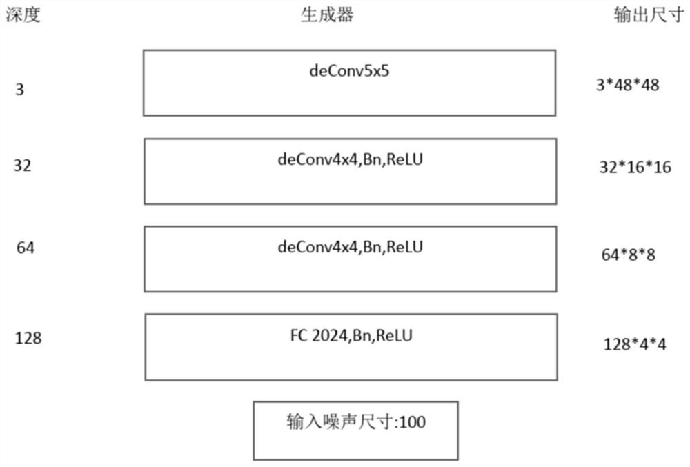
[0075] Step 3.1 The generator is composed of three upsampling parts based on the architecture of the fully convolutional neural network. For the consideration of the number and size of samples, the network designed in this paper only adds residuals after the second and third upsampling. The difference module is used to improve the learning ability and the quality of the generated image. The deconvolution is used to perform the upsampling operation of the image. The network first performs an upconvolution on the input 100-dimensional noise z, and the 100-dimensional noise can be regarded as 1*1* 100 data, and then generate a 128-dimensional 4*4 size feature map through deconvolution, and then pass two convolution kernels with a size of 4*4, a convolution stride of 2, and a deconvolution with a convolution kernel of 1. Upsampling is performed to generate 64-dimensional 8*8 and 32-dimensional 16*16 feature maps, respectively. After the 8*8 feature map, a two-layer convolution layer with a residual structure with a size of 3*3 is added for convolution. , after the feature map of 16*16, a four-layer convolution layer with a residual structure with a convolution kernel size of 3*3 is added for convolution, and finally the convolution kernel size is 5*5 and the convolution step size is 3. After upsampling, it is restored to a 48*48*3 generated image. After each convolutional layer in the network, a BN batch normalization layer is added and ReLu is used as the activation function. The last layer uses the tanh activation function and the Wasserstein distance as the loss. Function, generator Wasserstein distance definition derivation see step 3.2.
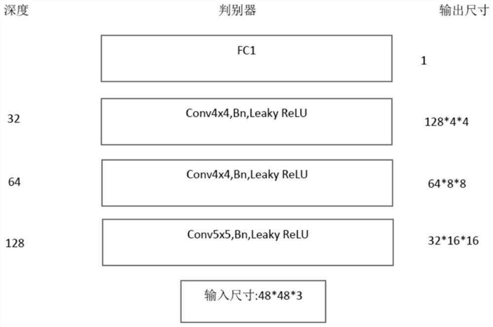
[0076] Step 3.2 Write the discriminator. The discriminator is divided into three downsampling modules, which is the inverse structure of the generator. The input is an image of 48*48*3. After downsampling and convolution to a 128-dimensional feature map, the output is classified through the fully connected layer. Discrimination, in the use of the activation function, the first three layers use leaky ReLu as the activation function, and the last layer uses the Wasserstein distance as the loss function for regression, where the Wasserstein distance is defined as follows:
[0077]
[0078] P data and P g respectively describe the distribution of real data and generated data, W(P data , P g ) represents the Wasserstein distance between the real data distribution and the generated data distribution, is P data and P g the set of combined joint distributions where each marginal distribution is P data and P g A joint distribution of , and for a subset γ joint distribution, a sample pair (x, y) can be randomly sampled from the sample pair (x, y) ~ γ that conform to the γ distribution, corresponding to the real sample and Generate a sample, and by calculating the distance ||x-y|| of the pair of samples, you can calculate the distance expectation E of the sample under the γ distribution (x,y)~γ [||x-y||], where ||x-y|| is the Euclidean distance for x and y, when x and y are image matrices, it is the sum of the squares of the differences of all elements of the matrix, for all possible γ-distributed samples Sum the expectations, inf indicates that these sets are taken to the lower bound, that is, the minimum value of the Euclidean distance for (x, y) of all available γ samples, as the distribution P data and P g Wasserstein distance between. This formula is used in the generator and discriminator, which can be substituted into P data Real data set and P g Generate the distance between the data sets and use this as a loss function to optimize the network. Since the γ distribution in this definition cannot be directly obtained, the next step needs to be derived.
[0079] It can be written in the following form according to the Kantorovich-Rubinstein duality theory, and the proof process is skipped:
[0080]
[0081] This formula is used to calculate the Wasserstein distance between the real sample data in the test set and the sample data generated by the generator. Here, the concept of Lipschitz continuity is introduced. Lipschitz continuity means that a constraint is imposed on a continuous function f, and its derivative function is The absolute value cannot exceed K, K≥0, which is mathematically defined as:
[0082] |f(x 1 )-f(x 2 )|≤K|x 1 -x 2 |
[0083] x 1 and x 2 In the formula, any two points on the f function are represented, and the Lipschitz constant of f is called K. In the formula ||f|| L is the Lipschitz constant of the function f, sup means to find The supremum of the expected difference between the two is the maximum value. In the formula, f means that the neural network maps the input x, which includes the input x~P from the real data. data and the input x ~ P from the network generated data g , the formula indicates that for a network function f that satisfies Lipschitz continuity, the Wasserstein distance is the result of the two mappings after using the network to map f to its input data x x~Pdata f(x) and x~Pg After f(x) is calculated, the difference is made, and its supremum, which is the maximum value, is taken and divided by K. In this method, ω represents the parameter matrix of all convolutional layers in the neural network, f represents the neural network, and x~P data Represents a sample image from the training data sample set, x~P g represents a sample image from the set of generated data samples, for the discriminator, x 1 and x 2 is the real image data for any test set, for the generator, x 1 and x 2 is a random 100-dimensional Gaussian noise, the formula can be approximately deformed into the following solution form:
[0084]
[0085] The formula indicates that K times the Wasserstein distance between the generated data and the real data is the neural network f with the network parameter ω for the real data and the generated data. ω The output under the mapping is expected to be the difference and the maximum value is obtained.
[0086] From this, the generator G loss function formula can be derived:
[0087]
[0088] Discriminator D loss function formula:
[0089]
[0090] where L G represents the loss function of the generator, L D represents the loss function of the discriminator, f ω (x) represents the mapping of the neural network with the parameter matrix ω to the input x. In the actual network, the generator input is 100-dimensional noise, the discriminator input is a 48*48 three-channel spore image, and ω is the network convolution matrix parameter , Find the mathematical expectation for the resulting pixel matrix mapping for a sample x of generated data input. Find the expectation for the sample x given by the real data after matrix mapping. generator L G The loss function is to take the negative number after the expectation of the generated data sample, and the discriminator L D The loss function is expressed as the expected difference between the generated data and the original real data, max indicates the maximum value of the expected difference obtained for different inputs x that meet the qualification conditions, and the value of K is 1 in this method. Spectral normalization is used in step 3.3 to make the network function f ω (x) Satisfy the Lipschitz continuity condition to use the Wasserstein distance as the loss function.
[0091] Step 3.3 Spectrally normalize the network parameters of the generator and the discriminator to satisfy the Lipschitz continuity condition in the Wasserstein distance. For a neural network, each layer can be regarded as a linear function, and each layer contains The parameters of multiple neurons and multi-layer neurons constitute the neural network parameter matrix W. When using the Wasserstein distance, Lipschitz continuity needs to be satisfied. The matrix mapping is a linear mapping. When the continuous condition is satisfied, only the zero point needs to be used. If its slope is less than K, the slope of the linear function represented by its matrix is less than K everywhere, and the continuous condition can be satisfied. For the discriminator, the input x represents the real data of the test set, and for the generator, the input x represents the input 100-dimensional Noise data, the calculation formula of the spectral norm of the network parameter matrix is as follows:
[0092]
[0093] where ||W|| 2 is the spectral norm of the matrix W, ||x|| 2 is the spectral norm of the input data x, which is the square root value of the largest eigenroot of the product of the transposed conjugate matrix of x and the matrix x, ||Wx|| 2 is the spectral norm of the output matrix obtained after the linear mapping of the network W, and is the square root value of the largest eigenroot of the product of the transposed conjugate matrix of the matrix Wx and the matrix Wx, and max represents the value of all input x that is not 0. The obtained W spectral norm takes the maximum value. Since the parameters of W will be initialized randomly at the beginning of network training, they cannot be obtained directly. The above method needs to be used to solve the problem. At this time, all parameters in the matrix W are spectrally normalized. Spectral Normalization, W SN Represents the normalized matrix W,:
[0094]
[0095] The spectral norm of W can be reduced to 1, that is, the spectral norm of each convolutional layer parameter matrix is also 1. At this time, the mapping relationship of any n-th layer network is W n , x, y are any two network inputs, the network input of the generator is 100-dimensional noise, and the network input of the discriminator is the real data of the test set, which has the following relationship:
[0096]
[0097] In this case, corresponding to the Lipschitz continuity |f(x 1 )-f(x 2 )|≤K|x 1 -x 2 | condition, and it can be known that K=1 at this time. If the normal algorithm process is used, it takes a lot of time and calculation to calculate the spectral norm of the network convolution layer matrix. Therefore, this method adopts a fast estimation spectral norm algorithm, the power iteration method to calculate the spectral norm estimate. The following are the steps of the power iteration method, where W is the network parameter matrix, (W) T is the transpose of the matrix, μ is an initialization matrix variable, its dimension and size are consistent with the W matrix, and the initial value of all elements of the matrix is 0:
[0098] Step1. Use a Gaussian function with a mean of 0 and a variance of 1 to generate a random Gaussian matrix variable ν 0 , which is used for iterative and repeated operations in Step2, iterating to the kth time, and its upper right corner becomes k, that is, ν k , its dimension and matrix size are the same as the W network parameter matrix, and the matrix parameter value is a Gaussian function with a mean value of 0 and a variance of 1 to generate.
[0099] Step2. Repeat the following operations for k times. In the experiment, k is the number of training times required for the stable convergence of the network loss function. The value of the network loss function will fluctuate and decrease with the training. When the change of the function value does not exceed 2% of its own value, you can It is determined to be convergent, which is set to 1000 in the experiment of this method, that is, the network can be trained for 1000 times to achieve a stable convergence state. In fact, it can be determined according to the number of training times required for the loss function to converge and stabilize during the training process of different data pictures. μ k and ν k represents the μ and ν matrices after the kth iteration.
[0100] let μ k ←Wν k , for μ k To regularize:
[0101] Let n k ←(W) T μ k , to n k To regularize:
[0102] Step3.||W|| 2 =(μ k ) T Wv k
[0103] ||μ k ||, ||ν k || is the pair matrix μ k and ν k The regularization operation is performed, that is, all elements in the matrix are squared and summed, and then the root sign is opened. The steps in Step2 need to be repeated k times. When the iteration reaches the kth, the step indicates that the Multiply the network parameter matrix W by the matrix ν, and assign its value to the matrix μ of the k-th iteration process k , and then for μ k After regularization, the resulting μ k Transpose W of Left Multiply Network Parameter Matrix T and assign its value to the matrix μ k , then for ν k Carry out the regularization operation, after iterating until the network loss function value converges stably, μ k is the eigenvector corresponding to the spectral norm of the matrix. Finally, in Step 3, multiply the matrix W to the left by μ k The transpose of and right-multiplying the matrix ν k The spectral norm of W can be obtained, and in actual training, as long as an iterative operation is performed after each training process, the estimation of the singular value can be solved more and more toward the final value with the training of the network. After the spectral norm of W, spectrally normalize the parameters in the matrix.
[0104] Step 3.4 Crop the data in the training set, and use a fixed-size crop frame to crop out a picture containing only a single target spore in each picture. A target powdery mildew spore.
[0105] In step 3.5, the obtained images are trained, and the RmsProp algorithm is used to optimize the loss function to generate a specified number of spore images.
[0106] Step 3.6 Screen the generated spore pictures. The original wheat powdery mildew spores are elliptical and light-colored spores with an aspect ratio of 1.5-2. Select the spore pictures that are similar in color and shape to the original wheat powdery mildew spores, and cover the original wheat powdery mildew spores. Cropped part of the picture to get a new batch of wheat powdery mildew spore pictures for data enhancement.
[0107] Step 4. Build an image segmentation model, add a pyramid pooling module and encoder-decoder connection structure to the encoder-decoder structure, and train the enhanced data obtained in steps 2 and 3 and the original training set data.
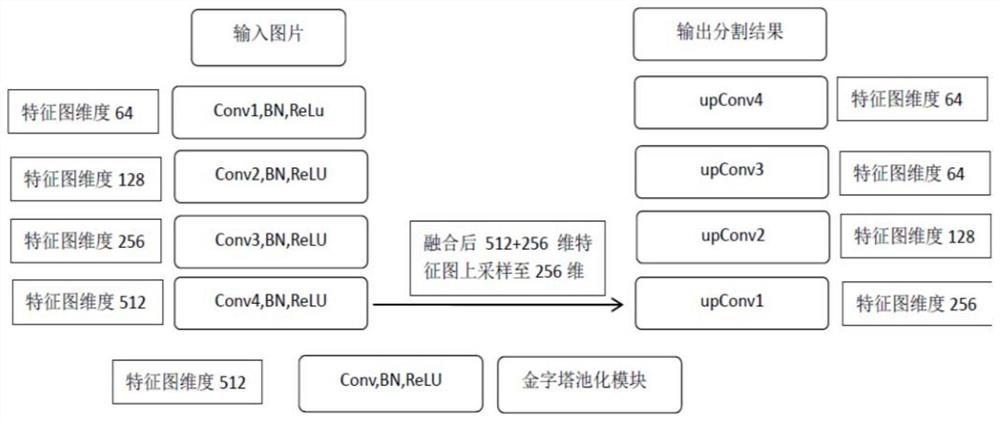
[0108] Step 4.1 Build an encoder-decoder network architecture. The encoder is a four-layer convolution downsampling, and the input is a normalized 256*256 image. Each layer uses a volume of 3*3 and a stride of 1. Accumulation kernel, the first layer of the network convolves the 3-channel 256*256 image into a 64*128*128 feature map, the second layer of convolution generates a 128*64*64 feature map, and the third layer of convolution generates 256 *32*32 feature map, the fourth layer of convolution generates a 512*16*16 512-dimensional feature map to extract feature information at different levels. The decoder is up-sampling with five layers of deconvolution, and uses the padding operation to supplement the edges, so that the original size can be restored, corresponding to the encoder.
[0109] Step 4.2 Add a connection structure between the fourth convolutional layer of the encoder and the convolutional layer of the decoder, and deconvolve the encoder convolutional feature matrix of the fourth layer and the fifth layer of the decoder to the fourth layer. After the feature matrix information is fused by the matrix dimensions, a convolution upsampling is performed again.
[0110]Step 4.3 Add the pyramid pooling module after the fifth convolutional layer of the encoder. Compared with the pyramid pooling network, this module pools and fuses the multi-layer feature maps with a single step size. The layer feature map is pooled with different steps. The size of the pooled convolution kernel is 2*2, and the pooled convolution with the step size of 2, 4, 6, and 13 is performed, so that the feature size of 16*16 can be used. In the figure, multi-scale feature combinations are generated to extract multi-scale features. Combined with the connection structure of the fourth layer, the feature extraction and learning effect of small targets can be effectively improved.
[0111] Step 4.4 trains the enhanced data obtained in step 2 and step 3 and the original training set data.
[0112] Step 5: Test the model generated by training on the test set, and use the model with the highest miou index as the result. miou is calculated as follows:
[0113]
[0114] where k+1 represents the number of categories including the background, p ij represents the number of pixels whose true value is i and is misclassified as j, then p ii represents the number of pixels of class i that are correctly predicted, p ji Represents the number of pixels with true value j that are misclassified as i.
[0115] The above embodiments are only exemplary embodiments of the present invention, and are not intended to limit the present invention, and the protection scope of the present invention is defined by the claims. Those skilled in the art can make various modifications or equivalent replacements to the present invention within the spirit and protection scope of the present invention, and such modifications or equivalent replacements should also be regarded as falling within the protection scope of the present invention.