Method and system for predicting air-to-surface target missile
Inactive Publication Date: 2009-04-02
NAT TAIWAN UNIV
7 Cites 12 Cited by
AI-Extracted Technical Summary
Problems solved by technology
However, if the trajectory prediction for the target missile has a large error, such as the aforementioned extended Kalman filer, or requi...
Benefits of technology
[0031]The techniques used by the present invention to solve the conventional problems are to deploy plural sensors at various locations for receiving echoed wave signals from the target missile, use the hybrid FSK/LFM unit to receive the signals and compute the relative distance and relative velocity of the target missile, use the two-stage Kalman filter to filter the computed relative distance and relative velocity to obtain the relative distance, relative velocity and relative acceleration of the target missile, and finally trilaterate by using the relative distance, relative velocity and relative acceleration of the target missile from each two-stage Kalman filter to obtain the components of location, velocity and acceleration along x, y, and z directions. The trilaertation module can further connect to plural one-stage Kalman filters to receive the location, velocity, and acceleration along each direction computed by the trilateration module to speed up the convergence.
[0032]The system and method of the present invention using FSK/LFM hybrid signal, two-stage Kalman filters, trilateration can effectively defend against the noise and a...
Abstract
A method and system for predicting a trajectory of an air-to-surface target missile is provided, including detecting a plurality of echo wave signals from the target missile through a plurality of sensors deployed at various locations relative to the target missile, extracting at least one range distance and at least one radial velocity, respectively, from the detected echo wave signals from the sensors by using a hybrid FSK/LFM unit, using a two-stage Kalman filter to filter the computed range distance and radial velocity to obtain a relative distance, a relative velocity and a relative acceleration, respectively, of the target missile, and finally applying trilateration on the relative distance, relative velocity and relative acceleration of the target missile from each two-stage Kalman filter to obtain a location, velocity and acceleration along the x, y, z directions.
Application Domain
Radio wave reradiation/reflection
Technology Topic
Relative velocityTrilateration +7
Image
Examples
- Experimental program(1)
Example
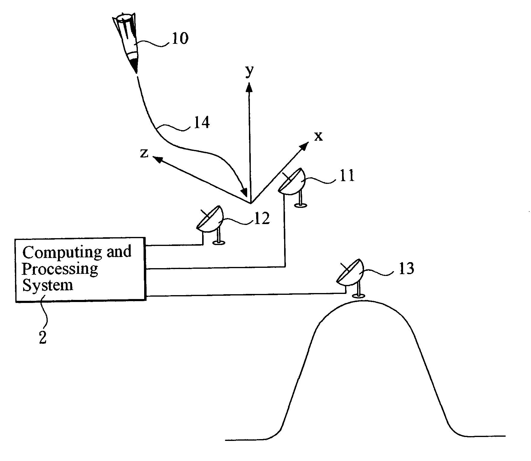
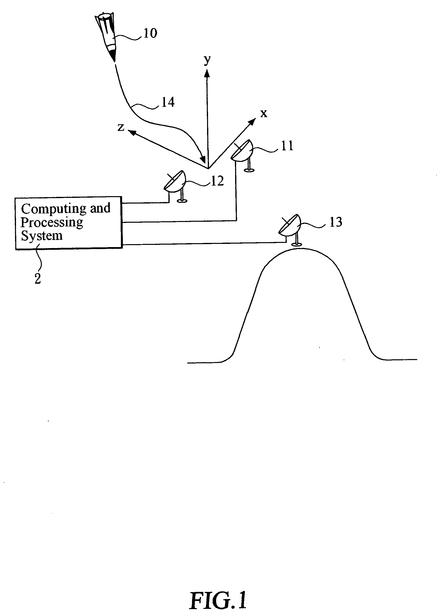
[0050]With reference to the drawings and in particular to FIG. 1, which shows a schematic view of a scenario in which a target missile attacking a field deployed with three sensors, the target missile 10 is a missile fired by the enemy and is thus the target for interception by a missile defense system.
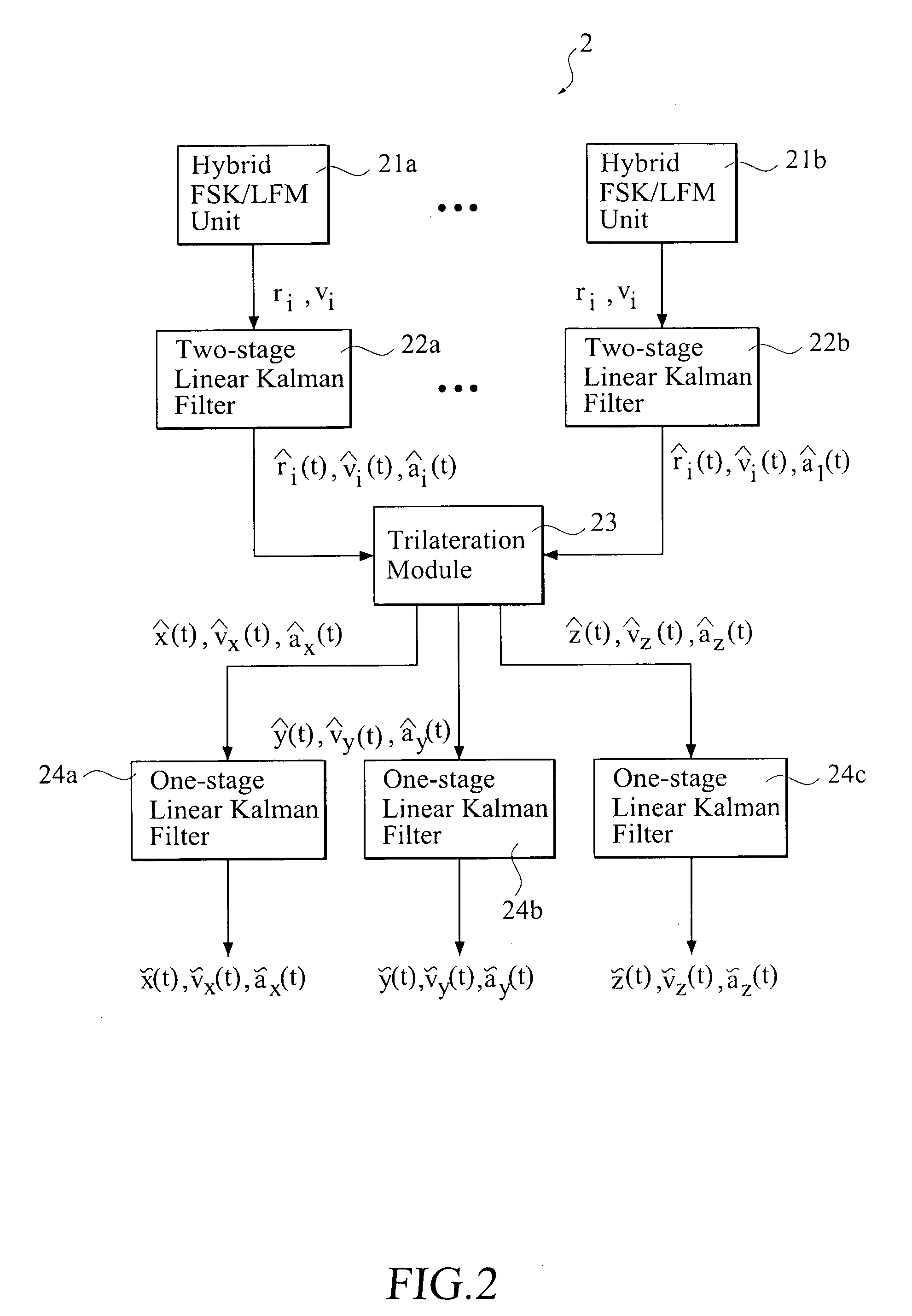
[0051]A first sensor 11, a second sensor 12, and a third sensor 13 are the devices, such as radar, for transmitting the detection signal and receiving the signal echoed from the target missile 10. The sensors 11, 12, 13 cover the field that is under attack by the target missile 10. The echo signals received by the sensors 11, 12, 13 are fed to a computing and processing system 2. Based on a pre-set algorithm, the computing and processing system 2 uses the echo signals to predict, i.e., compute, a trajectory 14 of the target missile 10.
[0052]Assume the target missile 10 moves with a fixed acceleration:
atx(t)=atx(0);
aty(t)=aty(0); and
atz(t)=atz(0),
where atx(0), aty(0) and atz(0) are initial acceleration. The integral of the initial acceleration is the velocity of the target missile 10.
v tx ( t ) = ∫ 0 t a tx ( τ ) τ = v tx ( 0 ) + a tx ( 0 ) t v ty ( t ) = ∫ 0 t a ty ( τ ) τ = v ty ( 0 ) + a ty ( 0 ) t v tz ( t ) = ∫ 0 t a tz ( τ ) τ = v tz ( 0 ) + a tz ( 0 ) t
where vtx(0), vty(0) and vtz(0) are the initial velocity. The integral of the velocity is the trajectory of the target missile 10
x t ( t ) = ∫ 0 t v t ( τ ) τ = x t ( 0 ) + v tx ( 0 ) t + 1 2 a tx ( 0 ) t 2 y t ( t ) = ∫ 0 t v ty ( τ ) τ = y t ( 0 ) + v ty ( 0 ) t + 1 2 a ty ( 0 ) t 2 z t ( t ) = ∫ 0 t v tz ( τ ) τ = z tz ( 0 ) + v tz ( 0 ) += t + 1 2 a tz ( 0 ) t 2
where xt(0), yt(0) and zt(0) are the initial coordinates.
[0053]In general, a missile can reach a maximum velocity of 1,360 m/s and a maximum g-load of 40 g. Assume that the target missile is initially located at xt(0)=0 m, yt(0)=6,000 m, and zt(0)=8,000 m, moving with vtx(0)=0 m/s, vty(0)=0 m/s, vtz(0)=−200 m/s, atx(0)=0 m/s2, aty(0)=−200 m/s2, and atz(0)=−300 m/s2.
[0054]A sensor can measure the radial distance and velocity as
r i ( t ) = [ x t ( t ) - x i ] 2 + [ y t ( t ) - y i ] 2 + [ z t ( t ) - z i ] 2 v i ( t ) = x t ( t ) - x i r i ( t ) v tx ( t ) + y t ( t ) - y i r i ( t ) v ty ( t ) + z t ( t ) - z i r i ( t ) v tz ( t )
where the subscript i refers to the i-th sensor.
[0055]FIG. 2 shows a schematic view of a preferred embodiment of a computing and processing system 2 of FIG. 1, including the combination of two-stage and one-stage Kalman filters to estimate the kinetic parameters, such as location, velocity and acceleration of the target.
[0056]The computing and processing system 2 includes a plurality of hybrid FSK/LFM units 21a, 21b for receiving the frequency-shift keying (FSK) and linear frequency modulation (LFM) hybrid signals echoed by the target missile 10 to obtain the distance ri and the radial velocity vi of target missile 10. The hybrid FSK/LFM units 21a, 21b are connected respectively to two-stage Kalman filters 22a, 22b for estimating {circumflex over (r)}i(t), {circumflex over (v)}i(t) and âi(t).
[0057]The {circumflex over (r)}i(t), {circumflex over (v)}i(t) and âi(t) generated by the two-stage Kalman filters 22a, 22b are transmitted to a trilateration module 23 to compute and determine {circumflex over (x)}(t), ŷ(t), {circumflex over (z)}(t), {circumflex over (v)}x(t), {circumflex over (v)}y(t), {circumflex over (v)}z(t), {circumflex over (0)}ax(t), ây(t) and âz(t).
[0058]The output of the trilateration module 23 is connected respectively to three one-stage linear Kalman filters 24a, 24b, 24c. The {circumflex over (x)}(t), {circumflex over (v)}x(t), âx(t) signals generated by the trilateration module 23 are sent to the one-stage Kalman filter 24a to generate {tilde over (x)}(t), {tilde over (v)}x(t), ãx(t). The ŷ(t), {circumflex over (v)}y(t), ây(t) signals generated by the trilateration module 23 are sent to the one-stage Kalman filter 24b to generate {tilde over (y)}(t), {tilde over (v)}y(t), ãy(t). The {circumflex over (z)}(t), {circumflex over (v)}z(t), ̂az(t) signals generated by the trilateration module 23 are sent to the one-stage Kalman filter 24c to generate {tilde over (z)}(t), {tilde over (v)}z(t), ãz(t).
[0059]FIG. 3 shows a flowchart of the method for predicting a trajectory of an air-to-surface missile of the present invention. The execution of the method of the present invention includes the use of a pluralilty of sensors deployed at various locations to detect the echoed wave signals from the target missile, as step 101, and followed by the following steps:
[0060](a) step 102: using the hybrid FSK/LFM units 21a, 21b to extract a range distance ri and a radial velocity vi from the echo hybrid FSK/LFM signal echoed from the target missile to the i-th sensor;
[0061](b) step 103: using the two-stage linear Kalman filters 22a, 22b to filter the range distance ri and radial velocity vi computed by the hybrid FSK/LFM units 21a, 21b to estimate the relative distance {circumflex over (r)}i, relative velocity {circumflex over (v)}i, and relative acceleration âi of the target missile;
[0062](c) step 104: using the trilateration module 23 to apply trilateration on the relative distance {circumflex over (r)}i, relative velocity {circumflex over (v)}i, and relative acceleration âi of the target missile estimated by each of the two-stage linear Kalman filters 22a, 22b to obtain the components of the location, velocity and acceleration of the target missile along the x, y, z directions, i.e., {circumflex over (x)}(t), ŷ(t), {circumflex over (z)}(t), {circumflex over (v)}x(t), {circumflex over (v)}y(t), {circumflex over (v)}z(t), âx(t), ây(t) and âz(t); and
[0063](d) step 105: using the three one-stage linear Kalman filters 24a, 24b, 24c to receive respectively the signals along each direction, i.e., {circumflex over (x)}(t), ŷ(t), {circumflex over (z)}(t), {circumflex over (v)}x(t), {circumflex over (v)}y(t), {circumflex over (v)}z(t), âx(t), ây(t) and âz(t), generated by the trilateration module 23.
[0064]The computing and processing steps are further described as follows.
[0065](1) Hyrbid FSK and LFM
[0066]FIG. 4 shows a schematic view of the frequency variation of signals of linear frequency modulation (LFM), where along the x-axis TLFM is the period, along the y-axis f(t), fr(t) are the frequency, and Bsweep is the bandwidth.
[0067]FIG. 4A shows a schematic view of frequency variation of FSK/LFM hybrid signals, where the frequency variations of two LFM signals have positive slopes SA and SB, respectively. To simplify the description, assume that SA and SB are both equal to S. 2N samples are taken with interval τ=TLFM/2N. The difference of frequency of the second signal measured at t=2nτ and that of the first signal measured at t=(2n−1)τ is fshift=fB(0)−fA(0)+Sτ. The frequency increment over 2τ is finc=Bsweep/N.
[0068]The difference between the frequency of the echo signal and that of the transmitted signal is Δf=frA(t)−fA(t). Let s=ΔfTLFM, then during the 0 LFM interval:
S = T TLFM [ f rA ( t ) - f A ( t ) ] = T LFM { [ f 0 + s ( t - 2 r A c ) ] ( 1 - 2 v A c ) - ( f 0 + st ) } = T LFM [ - 2 v A c f A ( t ) - 2 sr A c ( 1 - 2 v A c ) ] ≃ T LFM [ - 2 s c r A - 2 f A ( t ) c v A ] ( 1 )
A signal target with given range distance r and velocity v renders fA(t)>>fB(t)−fA(t), and thus S=SA≈SB. Typical parameters are Bsweep=150 MHz, fB(t)−fA(t)=300 kHz, TLFM=256 ms and N=256.
[0069]The difference of phase of the second signal measured at t=2nτ and that of the first signal measured at t=(2n−1)τ is:
Δ ϕ = ϕ B - ϕ A = 4 π c { [ f B ( 0 ) + 2 ns τ - 2 sr B c ] ( 1 - 2 v B c ) r B - [ f A ( 0 ) + ( 2 n - 1 ) s τ - 2 sr A c ] ( 1 - 2 v A c ) r A } ≃ 4 π c { [ f B ( 0 ) + 2 ns τ - 2 sr B c ] r B - [ f A ( 0 ) + ( 2 n - 1 ) s τ - 2 sr A c ] r A } ≃ 4 π c f shift r A + 4 π c f B ( t ) v a τ ( 2 )
From equations (1) and (2), the following relation can be obtained:
[ r v ] = [ - 2 s / c - 2 f A ( t ) / c 4 π f shift / c 4 π f B ( t ) τ / c ] - 1 [ S Δ ϕ ] ( 3 )
Equations (1) and (2) can both be expressed as a line segment on the r-v plane, and the angle between the two line segments is:
θ = tan - 1 ( 4 π c f shift π 2 N Δ v ) - tan - 1 ( 1 2 Δ r 1 2 Δ v )
where Δr=c/4 Bsweep is the range resolution, and Δv=λ/4TLFM is the velocity resolution. Choose the frequency shift fshift=−finc/2, and the two line segments will be orthogonal to achieve the highest range and velocity accuracy.
[0070](2) Two-Stage Kalman Filter
[0071]The steps of a two-stage Kalman filter are summarized as follows:
G _ _ xf ′ [ n ] = K _ _ x ′ [ n n - 1 ] · H _ _ † [ n ] · { H _ _ [ n ] · K _ _ x ′ [ n n - 1 ] · H _ _ † [ n ] + Q _ _ x 2 } - 1 ( 4 ) x _ ′ [ n n ] = x _ ′ [ n n - 1 ] + G _ _ xf ′ [ n ] · { y _ { n ] - H _ _ [ n ] · x _ ′ [ n n - 1 ] } ( 5 ) K _ _ x ɛ ′ [ n ] = K _ _ x ′ [ n n - 1 ] - G _ _ xf ′ [ n ] · H _ _ [ n ] · K _ _ x ′ [ n n - 1 ] ( 6 ) x _ ′ [ n n ] = A _ _ [ n + 1 ] · x _ ′ [ n n ] ( 7 ) K _ _ x ′ [ n + 1 n ] = A _ _ [ n + 1 ] · K _ _ x ɛ ′ [ n ] · A _ _ † [ n + 1 ] + Q _ _ x 1 ( 8 )
where x′ [n|n] is the filtered estimate of the state vector, x′[n+1|n] is the predicted estimate of the state vector, y[n] is the measurement vector, G′xf[n] is the Kalman gain matrix, K′xε[n] is the correlation matrix of x′[n|n], K′x[n+1|n] is the correlation matrix of x′[n+1|n], A[n] is the transition matrix, H[n] is the measurement matrix, Qx1 is the correlation matrix of he process noise vector, and Qx2 is the correlation matrix of the measurement vector.
[0072]The bias estimator is summarized as follows:
r _ [ n ] = y _ [ n ] - H _ _ [ n ] · x _ ′ [ n n - 1 ] G _ _ bf ′ [ n ] = K _ _ b ′ [ n n - 1 ] · S _ _ † [ n ] · { H _ _ [ n ] · K _ _ x ′ [ n n - 1 ] · H _ _ † [ n ] + S _ _ [ n ] · K _ _ b [ n n - 1 ] + S _ _ † [ n ] + Q _ _ x 2 } - 1 ( 9 ) b _ ^ [ n n ] = b _ ^ [ n n - 1 ] + G _ _ bf [ n ] · { r _ [ n ] - S _ _ [ n ] · b _ ^ [ n n - 1 ] } ( 10 ) K _ _ b ɛ [ n ] = K _ _ b [ n n - 1 ] - G _ _ bf [ n ] · S _ _ [ n ] · K _ _ b [ n n - 1 ] ( 11 ) b _ ^ [ n n - 1 ] = b _ ^ [ n - 1 n - 1 ] ( 12 ) K _ _ b [ n n - 1 ] = K _ _ b ɛ [ n - 1 ] ( 13 )
where r[n] is the measurement residual of the bias-free estimator, {circumflex over (b)}[n|n] is the filtered estimate of the bias state vector, {circumflex over (b)}[n|n−1] is the predicted estimate of the bias state vector, Gbf [n] is the Kalman gain matrix of the bias estimator, Kbε [n] is the correlation matrix of {circumflex over (b)}[n|n], Kb[n|n−1] is the correlation matrix of {circumflex over (b)}[n|n−1], and S[n] is the sensitivity matrix. S[n] can be derived as:
U [n]= A [n]· V [n−1]+ B [n] (14)
V [n]= U [n]− G xf′[n]· S [n] (15)
S [n]= H [n]· U [n]+ D [n] (16)
where B[n] is the bias transition matrix, and D[n] is the bias measurement matrix.
[0073]In this two-stage Kalman filter, the measurement vector yi[n] and the dynamic state vector xi[n] associated with the i-th sensor are defined respectively as
y _ i [ n ] = [ r i [ n ] v i [ n ] ] , x _ i [ n ] = [ r ^ i [ n ] v ^ i [ n ] ]
and the bias vector is defined as
bi[n]=[âi[n]]
Thus, the state transition matrix Ai[n] and the bias transition matrix Bi[n] can be derived respectively as
A _ _ i [ n ] = [ 1 T p 0 1 ] , B _ _ i [ n ] = [ T p 2 / 2 T p ]
The measurement matrix Hi[n] is equal to an identity matrix of rank 2, and the bias measurement matrix is Dii[n]= 0.
[0074]The correlation matrix of the process noise vector can be expressed as
Qi1= Li·Qia·Li†
where
L _ _ i = [ T p 2 / 2 T p ] , Q _ _ ia = E { a 2 }
The inputs to this two-stage Kalman filter are the measurement data of ri and vi. Since no information on ai is available, the maximum acceleration of the missile, 40 g, is taken as the standard deviation, thus E{a2}=160,000 m2/s4.
[0075]The correlation matrix of the measurement noise vector can be expressed as:
Q _ _ i 2 = [ σ r 2 0 0 σ v 2 ]
Note that the first subscript in Qαβ indicates the α-th sensor. The standard deviation of range measurement is assumed σr=1 m, and the standard deviation of velocity measurement is assumed σv=3.35 m/s.
[0076]The initial values are xi′i[1|0]=[ri[0] vi[0]]t, Ki,x′ [1|0]= I2×2, bi′i [1|0]=[0]t, Ki,b′[1|0]= I1×1 and Vi[0]= Li.
[0077](3) Trilateration
[0078]Assume the i-th sensor is located at (xi, yi, zi), and the reflecting point of the target is located at ({circumflex over (x)}, ŷ, {circumflex over (z)}), moving with velocity ({circumflex over (v)}x, {circumflex over (v)}y, {circumflex over (v)}z). The outputs form the first two-stage Kalman filter are {circumflex over (r)}i, {circumflex over (v)}i and âi.
[0079]The radial ranges {circumflex over (r)}1, {circumflex over (r)}2 and {circumflex over (r)}3 from the three sensors to the target are
{circumflex over (r)}12=({circumflex over (x)}−x1)2+ŷ2+{circumflex over (z)}2 (17)
{circumflex over (r)}22=({circumflex over (x)}−x2)2+ŷ2+{circumflex over (z)}2 (18)
{circumflex over (r)}32={circumflex over (x)}2+(ŷ−y3)2+({circumflex over (z)}−z3) (19)
Note that y1=z1=y2=z2=x3=0. Eliminating ŷ and {circumflex over (z)} from equations (17) and (18) results in
r ^ 1 2 - ( x ^ - x 1 ) 2 = r 2 2 - ( x ^ - x 2 ) 2 x = x 1 2 - x 2 2 - r ^ 1 2 + r ^ 2 2 2 ( x 1 - x 2 ) ( 20 )
From equations (18) and (19), ŷ can be determined as
y ^ = - p 2 + p 2 2 - 4 p 1 p 3 2 p 1 ( 21 )
where
p 1 = 1 + y 3 2 z 3 2 , p 2 = - 2 p 4 y 3 z 3 p 3 = p 4 2 - r ^ 2 2 + ( x ^ - x 2 ) 2 p 4 = r ^ 2 2 - ( x ^ - x 2 ) 2 - r ^ 3 2 + x ^ 2 + y 3 2 + z 3 2 2 z 3
Then, {circumflex over (z)} can be determined as
z = p 4 - y ^ 3 z 3 y ^ ( 22 )
[0080]The radial velocity {circumflex over (v)}1, {circumflex over (v)}2 and {circumflex over (v)}3 are related to {circumflex over (v)}x, {circumflex over (v)}x and {circumflex over (v)}Z as
v ^ 1 = x ^ - x 1 r ^ 1 v ^ x + y ^ r ^ 1 v ^ y + z ^ r ^ 1 v ^ z v ^ 2 = x ^ - x 2 r ^ 2 v ^ x + y ^ r ^ 2 v ^ y + z ^ r ^ 2 v ^ z v ^ 3 = x ^ r ^ 3 v ^ x + y ^ - y 3 r ^ 3 v ^ y + z ^ - z 3 r ^ 3 v ^ z
or in the matrix form
[ v ^ x v ^ y v ^ z ] = L _ _ - 1 · [ v ^ 1 r ^ 1 v ^ 2 r ^ 2 v ^ 3 r ^ 3 ] ( 23 )
where
L _ _ = [ x ^ - x 1 y ^ z ^ x ^ - x 2 y ^ z ^ x ^ y ^ - y 3 z ^ - z 3 ]
Similarly, the acceleration âx, ây and âz are related to â1, â2 and â3 as
[ a ^ x a ^ y a ^ z ] = L _ _ - 1 · [ a ^ 1 r ^ 1 a ^ 2 r ^ 2 a ^ 3 r ^ 3 ] ( 24 )
[0081](4) One-Stage Kalman Filter
[0082]To speed up the convergence rate, the present invention uses another one-stage Kalman filter to speed up the estimation of the parameters. As the data processing of a linear Kalman filter in one direction is independent of the other two, the data associated with the x, y, and z components are processed separately.
[0083]The one-stage Kalman filter is summarized as follows:
R _ _ α [ n ] = C _ _ [ n ] · K _ _ [ n n - 1 ] · C _ _ † [ n ] + Q _ _ 2 ( 25 ) G _ _ [ n ] = K _ _ [ n n - 1 ] · C _ _ † [ n ] · R _ _ α - 1 [ n ] ( 26 ) α _ [ n ] = y _ [ n ] - C _ _ [ n ] · x ^ [ n n - 1 ] ( 27 ) x ^ [ n n ] = x ^ [ n n - 1 ] + G _ _ [ n ] · α _ [ n ] ( 28 ) x ^ [ n + 1 n ] = F _ _ [ n + 1 n ] · x ^ [ n n ] ( 29 ) K _ _ ɛ [ n ] = K _ _ [ n n - 1 ] - G _ _ [ n ] · C _ _ [ n ] · K _ _ [ n n - 1 ] ( 30 ) K _ _ [ n + 1 n ] = F _ _ [ n + 1 n ] · K _ _ ɛ [ n ] · F _ _ † [ n + 1 n ] + Q _ _ 1 ( 31 )
where α[n] is the innovation vector, {circumflex over (x)}[n|n] is the filtered estimate of the state vector, {circumflex over (x)}[n+1|n] is the predicted estimate of the state vector, ŷ[n] is the measurement vector, Rα[n] is the correlation matrix of α[n], G[n] is the Kalman gain, Kε=[n] is the correlation matrix of {circumflex over (x)}[n|n], K[n+1|n] is the correlation matrix of {circumflex over (x)}[n+1|n], C[n] is the measurement matrix, F[n+1|n] is the transition matrix, Q1 is the correlation matrix of the process noise vector, and Q2 is the correlation matrix of the measurement noise vector.
[0084]The measurement vector yβ[n] and the state vector xβ[n] of the one-stage Kalman filter associated with the β component are defined as
y _ β [ n ] = [ β ^ [ n ] v ^ β [ n ] a ^ β [ n ] ] , x _ β [ n ] = [ β ^ [ n ] v ^ β [ n ] a ^ β [ n ] ]
with β=x, y or z. The state transition matrix can be derived as
F _ _ β [ n + 1 ] n = [ 1 T p T p 2 / 2 0 1 T p 0 0 1 ]
The measurement matrix is Cβ[n]= I3×3. The correlation matrix of the process noise vector is Qβ1= 0. The correlation matrix of the measurement noise vector is assumed to be
Q _ _ β 2 = [ σ β 2 0 0 0 σ v β 2 0 0 0 σ a β 2 ]
The initial values are xβ[1|0]=[{circumflex over (β)}[0]{circumflex over (v)}β[0] {circumflex over (α)}β[0]]t and Kβ[1|0]=Ī3×3.
[0085](5) Combination of Two-Stage Kalman Filter and One-Stage Kalman Filter
[0086]FIGS. 5A-5I show the prediction errors of a simulation trial after steps 101-104. During 1,000 Tp≦t≦2,000 Tp the errors of x, y, and x are within 0.8 m, 4 m and 6 m, respectively, the errors of vx, vy, and vz are within 10 m/s, 20 m/s and 25 m/s, respectively, and the errors of ax, ay, and az, are within 1.3 m/s2, 199 m/s2 and 297 m/s2, respectively.
[0087]The standard deviations of the kinetic parameters at t=2,000 Tp obtained by Monte Carlo simulation with ensemble size M=100 are
σ ^ x = 1 M ∑ n = 1 M ( x ^ - x ) 2 = 0.377 m σ ^ y = 1 M ∑ n = 1 M ( y ^ - y ) 2 = 3.187 m σ ^ z = 1 M ∑ n = 1 M ( z ^ - z ) 2 = 4.139 m σ ^ v x = 1 M ∑ n = 1 M ( v ^ x - v x ) 2 = 5.82 m / s σ ^ v y = 1 M ∑ n = 1 M ( v ^ y - v y ) 2 = 13.235 m / s σ ^ v z = 1 M ∑ n = 1 M ( v ^ z - v z ) 2 = 11.2 m / s σ ^ a x = 1 M ∑ n = 1 M ( a ^ x - a x ) 2 = 0.55 m / s 2 σ ^ a y = 1 M ∑ n = 1 M ( a ^ y - a y ) 2 = 197.85 m / s 2 σ ^ a z = 1 M ∑ n = 1 M ( a ^ z - a z ) 2 = 295.838 m / s 2
Note that the prediction of acceleration takes a very long time to converge. The estimated acceleration is close to zero at t≦2,000 Tp, if the initial values of acceleration are set to zeros.
[0088]Assume the standard deviations in the correlation matrices of the measurement noise vectors Qx2, Qy2 and Qz2 for the second one-stage Kalman filter are σx=σy=σz=11 m, σvx=σvy=σvz=1 m/s and σax=σay=σaz=400 m/s2. The choice of parameters in the correlation matrices of the measurement noise vector turn out not to affect the simulation results obviously.
[0089]The one-stage Kalman filter in step 104 tends to decrease the convergence time in estimating the accelerations. FIGS. 6A-6I show the prediction errors using this one-stage Kalman filter. During 1,000 Tp≦t≦2,000 Tp, the errors of x, y, and x are within 1 m, 6 m and 10 m, respectively, the errors of vx, vy, and vz are within 2.2 m/s, 9 m/s and 10 m/s, respectively, and the errors of ax, ay, and az, are within 4 m/s2, 5 m/s2 and 7 m/s2, respectively.
[0090]The standard deviations of parameters at t=2,000 Tp obtained with ensemble size M=100 are
σ _ x = 1 M ∑ n = 1 M ( x _ - x ) 2 = 0.546 m σ _ y = 1 M ∑ n = 1 M ( y _ - y ) 2 = 4.807 m σ _ z = 1 M ∑ n = 1 M ( z _ - z ) 2 = 5.954 m σ _ v x = 1 M ∑ n = 1 M ( v _ x - v x ) 2 = 0.913 m / s σ _ v y = 1 M ∑ n = 1 M ( v _ y - v y ) 2 = 3.153 m / s σ _ v z = 1 M ∑ n = 1 M ( v _ z - v z ) 2 = 2.97 m / s σ _ a x = 1 M ∑ n = 1 M ( a _ x - a x ) 2 = 0.941 m / s 2 σ _ a y = 1 M ∑ n = 1 M ( a _ y - a y ) 2 = 2.302 m / s 2 σ _ a z = 1 M ∑ n = 1 M ( a _ z - a z ) 2 = 1.766 m / s 2
[0091]Note that the errors of x, y and z of the second Kalman filter are slightly larger than those of the first Kalman filter. However, the errors of vx, vy, vz, ax, ay and az of the second Kalman filter are smaller than those of the first Kalman filter, especially the ay and az components. After step 103, the errors of coordinates are small, but those of velocities and accelerations are relatively large. Thus, the second Kalman filter has more effect on velocities and accelerations than on the coordinates.
[0092]FIGS. 6A-6I show the prediction errors in step 104, Tp=1 ms, σx=σy=σz=1 m, σvx=σvy=σvz=1 m/s, and σax=σay=σaz=40 0 m/s2.
[0093]In practice, the target coordinates can be estimated by using the first Kalman filter, and the velocities and accelerations can be estimated by using the second Kalman filter.
[0094]FIG. 7 shows a schematic view of the procedure of using a conventional two-stage Kalman filter to estimate the target kinetic parameters. The first step is to determine the range ri using the LFM echoes from three sensors, then send these data to the two-stage Kalman filter to estimate {circumflex over (r)}i(t), {circumflex over (v)}i(t) and âi(t). The second step is to use trilateration in equations (20)-(24) to calculate {circumflex over (x)}(t), ŷ(t), {circumflex over (z)}(t), {circumflex over (v)}x(t), {circumflex over (v)}y(t), {circumflex over (v)}z(t), âx(t),ây(t) and âz(t).
[0095]FIGS. 8A-8I show the prediction errors using the two-stage Kalman filter, Tp=1 ms, σr=1 m, σvx=σvy=σvz=1 m/s and E{a2}=160,000 m2/s4. During 1,000 Tp≦t≦2,000 Tp, the errors of x, y, and z are within 2 m, 10 m and 10 m, respectively, the errors of vx, vy, and vz are within 15 m/s, 50 m/s and 50 m/s, respectively, and the errors of ax, ay, and az are within 0.002 m/s2, 200 m/s2 and 300 m/s2, respectively.
[0096]As shown in FIG. 8, the convergence time for predicting the acceleration is about 500 seconds. The errors of location, velocity and acceleration are larger than those of predicted by the present invention.
[0097]FIG. 9 shows the procedure of a conventional extended Kalman filter to estimate the target kinetic parameters. The first step is to determine the range ri and vi using the hybrid FSK/LFM echoes from three sensors, and then send these data to the extended Kalman filter to estimate {circumflex over (x)}(t), ŷ(t), {circumflex over (z)}(t), {circumflex over (v)}x(t), {circumflex over (v)}y(t), {circumflex over (v)}z(t), âx(t), ây(t) and âz(t).
[0098]FIGS. 10A-10I show the prediction errors using the extended Kalman filter Tp=1 ms, σr=11 m, σv=1 m/s, and σa=400 m/s2.
[0099]During 1,000 Tp≦t≦2,000 Tp, the errors of x, y, and z are within 0.6 m, 85 m and 110 m, respectively, the errors of vx, vy, and vz are within 1.2 m/s, 70 m/s and 150 m/s, respectively, and the errors of ax, ay, and az are within 1.6 m/s2, 90 m/s2 and 170 m/s2, respectively. These errors are larger than those of the present invention.
[0100]FIG. 11 shows the difference between the acceleration of the moving target and the received data from the extended Kalman filter. If only the measurement data from one sensor is used in the extended Kalman filter, the estimated acceleration will be the projection of the real value in the direction from the sensor to the target. As shown in FIG. 11, the following can be obtained
a ^ x = x ^ - x i r i a i ( t ) a ^ y = y ^ - y i r i a i ( t ) a ^ z = z ^ - z i r i a i ( t )
where x, y, z, ax, ay, and az are the values from the moving target to the reference point, âx, ây and âz are the estimated accelerations of the i-th sensor by using the extended Kalman filter, and ri is the observed range from the i-th sensor at (xi, yi, zi).
[0101]To determine the interception point, using Patriot as an example, which has the maximum range of 70 km and the ceiling of 24 km. When the target missile approaches (0, 4400, 4800) meter at t=4 s, it will fall within the impact range of the Patriot.
[0102]Table 1 shows the errors of predicted coordinates at t=4 s.
TABLE 1 Error of TS/OSKF TSLKF EKF x (m) 9.475 10.318 5.3 y (m) 23.268 478.351 222 z (m) 8.866 746.772 548
[0103]FIG. 12 shows the estimated target trajectories by the preferred embodiment of the present invention (represented by line -), the conventional two-stage linear Kalman filter (represented by line -.-) and the conventional extended Kalamn filter (represented by line - -:), respectively, and line o-o is the real target tradjectory, where x: t=2 s and ⋄t=4 s.
[0104]As shown in FIG. 12, the predicted error of the estimated target coordinates at t=4 s by using the present invention are ex=9.475 m, ey=23.268 m, and ez=8.866 m, the predicted error using the two-stage linear Kalman filter are ex=10.318 m, ey=478.351 m, and ex=746.772 m, and the predicted error using the extended Kalman filter are ex=5.3 m, ey=222 m, and ez=548 m. Note that the convergence time of the two-stage linear Kalman filter is very long, and the estimated accelerations are closer to zero. Thus, the predicted trajectory appears as a tangent to the original trajectory at t=2s. The error of the predicted coordinates at t=4s are summarized in the aforementioned Table 1. The predicted trajectory using the present invention is the closest to the actual trajectory.
[0105]While the invention has been described in connection with what is presently considered to the most practical and preferred embodiment, it is to be understood that the invention is not to be limited to the disclosed embodiment, but on the contrary, is intended to cover various modifications and equivalent arrangement included within the spirit and scope of the appended claims.
PUM


Description & Claims & Application Information
We can also present the details of the Description, Claims and Application information to help users get a comprehensive understanding of the technical details of the patent, such as background art, summary of invention, brief description of drawings, description of embodiments, and other original content. On the other hand, users can also determine the specific scope of protection of the technology through the list of claims; as well as understand the changes in the life cycle of the technology with the presentation of the patent timeline. Login to view more.
Similar technology patents
Imaging System Utilizing Illumination and Optical Modules Contained within Rotating Optical Platens
InactiveUS20070013971A1accurately locateoptimally focus
Owner:PIXON TECH CORP
Transmitter-receiver comprising an electronic chip
ActiveUS20200186260A1accurately locateeasily add
Owner:THE SWATCH GRP RES & DEVELONMENT LTD
Information diffusion prediction method and device
ActiveCN106372437Asmall sample sizefast prediction
Owner:BEIJING UNIV OF POSTS & TELECOMM
Method and system for providing indoor positioning service
Owner:NAVER CLOUD CORP
Circular Knitting Machine With Mounting Arrangement For Sinker Cams
Owner:MONARCH KNITTING MACHINERY
Daily throughput estimation system for semi-conductor manufacturing system
Owner:SHANGHAI JIAO TONG UNIV
HSMM and empirical model-based fuel cell fault prediction method
Owner:UNIV OF ELECTRONIC SCI & TECH OF CHINA
Classification and recommendation of technical efficacy words
- accurately locate
- fast prediction
System and method for two-dimensional keystone correction for aerial imaging
ActiveUS20060291744A1accurately locatenot computationally intensive
Owner:TEXAS INSTR INC
Base station and mobile terminal for location detection, and location detecting method
InactiveUS20050128142A1accurately locate
Owner:ELECTRONICS & TELECOMM RES INST
HSMM and empirical model-based fuel cell fault prediction method
Owner:UNIV OF ELECTRONIC SCI & TECH OF CHINA
Daily throughput estimation system for semi-conductor manufacturing system
Owner:SHANGHAI JIAO TONG UNIV
Information diffusion prediction method and device
ActiveCN106372437Asmall sample sizefast prediction
Owner:BEIJING UNIV OF POSTS & TELECOMM