

Behavior Recognition Method Based on Joint Statistical Descriptor in Wavelet Domain
A recognition method and wavelet domain technology, applied in the field of video processing, can solve problems such as low feature dimension, unconsidered coefficient direction, relationship between coefficients, insufficient data coverage, etc., to achieve effective extraction and reduce impact
- Summary
- Abstract
- Description
- Claims
- Application Information
AI Technical Summary
Problems solved by technology
Method used
Image

Examples
Embodiment Construction
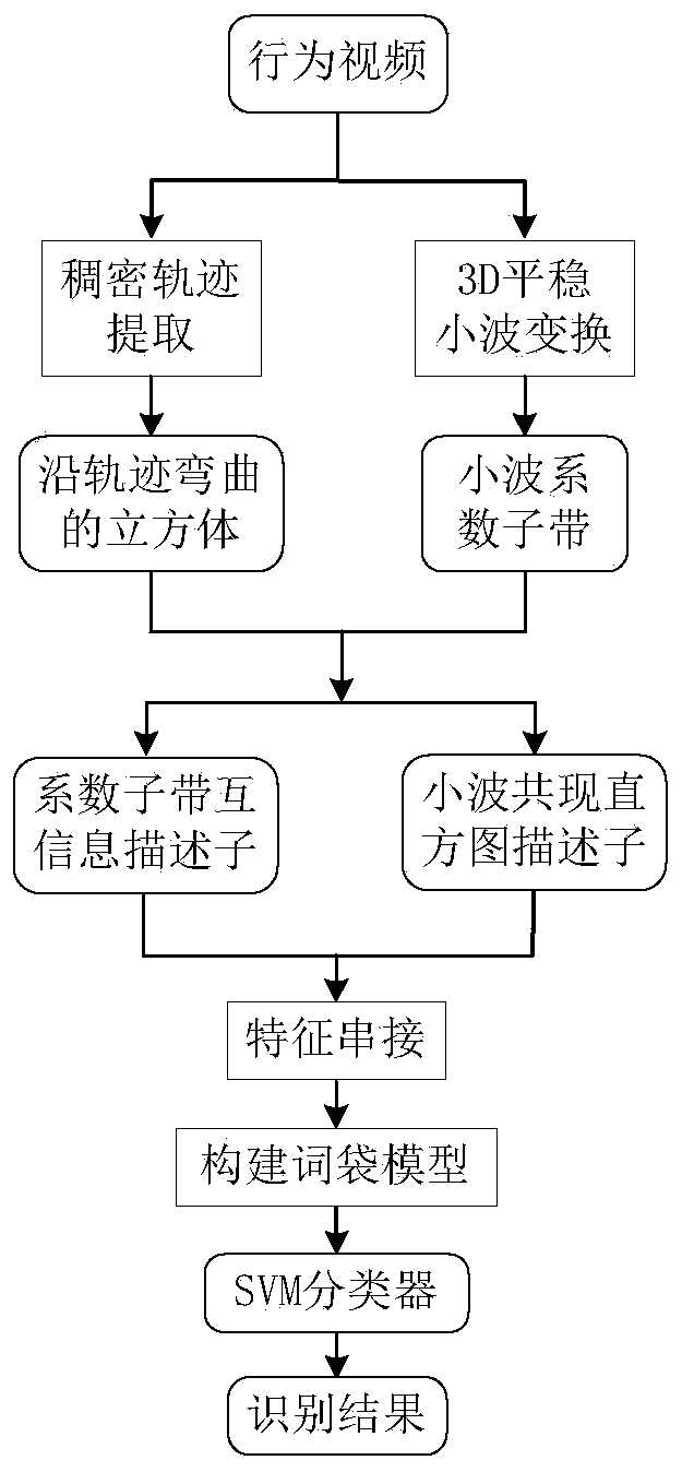
[0027] refer to figure 1 , the behavior recognition method based on wavelet domain joint statistical descriptor of the present invention, the steps are as follows:
[0028] Step 1, conduct dense sampling on behavioral videos and extract dense trajectories of video sequences.
[0029] Common trajectory extraction methods include trajectory tracking based on KLT (Kanade-Lucas-Tomasi), trajectory tracking based on SIFT (Scale Invariant Feature Transform) descriptor matching, and trajectory tracking based on dense optical flow. The present invention adopts the trajectory tracking method based on dense optical flow proposed by Wang et al. in the article "Action recognition by dense trajectories" in 2011 to extract the motion trajectory of the action video. The steps are as follows:
[0030](1.1) Use a dense grid to densely sample the video in eight scale spaces in turn, and the scaling factor between each two scale spaces is The sampling interval is 5 pixels;
[0031] (1.2) Cal...
PUM
 Abstract
Description
Claims
Application Information