Ultrasound speckle reduction and image reconstruction using deep learning techniques
Active Publication Date: 2019-09-26
THE BOARD OF TRUSTEES OF THE LELAND STANFORD JUNIOR UNIV
0 Cites 6 Cited by
AI-Extracted Technical Summary
Problems solved by technology
However, in medical ultrasound imaging, echoes are generated by scattering sources that are smaller than the resolution of the imaging system.
These echoes from subresolution scatterers interfere stochastically, producing a strong multiplicative noise in the measured DAS output.
However, for the task of echogenicity estimation, speckle reduces the perceived resolution of the target and is largely treated as an undesirable noise that degrades diagnostic B-mode imaging.
However, improvements in speckle SNR are limited to √{square root over (N)} when spatial compounding with N uncorrelated images, with lesser improvements when the compounded images are correlat...
Method used
The minimization problem is typically solved using some form of gradient descent, an approach in which each of the parameters is iteratively updated to reduce the error:
[0032]In order to reconstruct desired B-mode images with a neural network, the network 100 is first trained using training data, i.e., a set of inputs and corresponding true outputs that can be compared to the network output using a loss function. The training process is designed to determine the optimal parameters θ* that minimize the error between an estimated image y output from the network and the true image y, as quantified by some loss function (y, ŷ):
[0047]Image resolution was measured using the following methodology. First, the system response to a transition between two regions of different echogenicities was measured, referred to as the edge spread function (ESF). Field II Pro was used to simulate a target wherein half the azimuthal field of view was a speckle region of constant echogenicity and the other half was an anechoic region. The resulting images were averaged axially and over 16 independent scatterer realizations to reduce noise. Next, the ESF was differentiated in the azimuthal dimension to produce a line spread function (LSF). Finally, the FWHM of the LSF was measured to obtain the image resolution.
[0050]The input to the network was a 64×64×32 dataset, where the last dimension corresponded to real and imaginary components of 16 subaperture signals. A conventional DAS envelope-detection reconstruction 116 generates a conventional B-mode image 118, which was concatenated to the output of the M-th block 108. The speckle-reduced B-mode image output 114 was obtained by applying one final 2D convolution 110 and squaring the result. As will be explained further below in relation to FIGS. 4A-C, concatenating the B-mode image 118 after the M-th convolutional block significantly enhances training. Although the input channel data 112 theoretically contain all of the raw information necessary to reconstruct a B-mode image 114, it appears that the concatenated B-mode image 118 served as a good initial estimate of echogenicity for the network to improve upon, rather than learning the reconstruction from scratch. The uncompressed B-mode image 118 is separately formed from the input data 112 using equation (1) and concatenated to the output of the M-th block 108, yielding a data array of size P×Q×(F+1). The final convolution filter 110 of size 1×1×(F+1) was used to produce the output image 114 of size P×Q×1 that was subsequently squared on a pixel-wise basis to yield positive values of echogenicity. The fully convolutional nature of the network allowed echogenicity estimation on a pixel-wise basis. Unless otherwise specified, the default parameters for the networks were M=16 convolution blocks with F=32 filters per layer. Pooling layers and dropout were not utilized.
[0053]We performed hyperparameter tuning of the learning rates, batch size, and both l1 and l2 regularization of filter weights to achieve optimal performance using an independent validation dataset that was separate from all other datasets. The final hyperparameters used are tabulated in Table 2.
[0055]All testing was performed using a neural network with a depth of 16 blocks, a width of 32 filters, and trained to minimize the *Mix loss function for 30 training epochs unless otherwise indicated. The speckle reduction performance of the network was compared against those of receive spatial compounding and optimized Bayesian nonlocal means (OBNLM). Spatial compounding was implemented on receive by performing DAS beamforming and envelope detection independently on four non-overlapping subapertures and summing the result. The OBNLM algorithm was applied to images that were beamformed according to equation (1) using the publicly available MATLAB implementation provided by the authors of this algorithm. The default parameter values provided by the authors were used (M=7, α=3, h=0.7).
[0058]Generalizability to clinical imaging conditions was assessed in vivo in the kidney of a healthy 58-year-old male volunteer and in the liver of a 68-year-old female who had a focal lesion with a surrounding fluid capsule. Channel datasets were acquired with a modified Siemens S2000 scanner using a Siemens 4C1 transducer. Pulse-inversion harmonic imaging was performed using focused transmissions at 1.82 MHz. Due to technical limitations, the channel signals were obtained for only 64 (out of 192) elements in a sector of 54 (out of 192) beams. The remaining beams were acquired using the full aperture using conventional DAS. The 64 receive channel signals were beamformed into 16 subaperture signals prior to being input into the neural network. For this particular dataset only, a partially-trained network (15 epochs rather than 30) was used to evaluate speckle reduction to avoid overfitting. Image quality was assessed using contrast, CNR, and SNR of the liver lesion vs. the surrounding fluid, with the ROIs ...
Benefits of technology
[0012]In one aspect, the present invention provides a method for ultrasound image reconstruction using a neural network. A method is provided for reconstructing speckle-reduced B-mode images directly from real-time ultrasound channel signals using...
Abstract
Ultrasound B-mode images are reconstructed directly from transducer channel signals using a convolutional neural network (CNN). The CNN is trained with a dataset including, as inputs, simulated transducer array channel signals containing simulated speckle and, as outputs, corresponding simulated speckle-free B-mode ground truth images. After training, measured real-time RF signals taken directly from an ultrasound transducer array elements prior to summation are input to the CNN and processed by the CNN to generate as output an estimated real-time B-mode image with reduced speckle.
Application Domain
Reconstruction from projectionOrgan movement/changes detection +8
Technology Topic
VIT signalsData set +12
Image
Examples
- Experimental program(1)
Example
Problem Formulation
[0030]Consider a vectorized grid of P×Q field points (also referred to as “pixels”) with true echogenicities yϵ PQ. Let Xϵ PQ×N denote the demodulated analytic signals captured by the N elements of a transducer array after applying the appropriate time delays to focus the array at each of the field points. In B-mode image reconstruction, y is estimated from X using some function ƒ(X)=ŷ.
[0031]In the traditional delay-and-sum (DAS) technique, y is estimated as the absolute value of the channel sum:
ŷ=ƒDAS(X)=|X1|, (1)
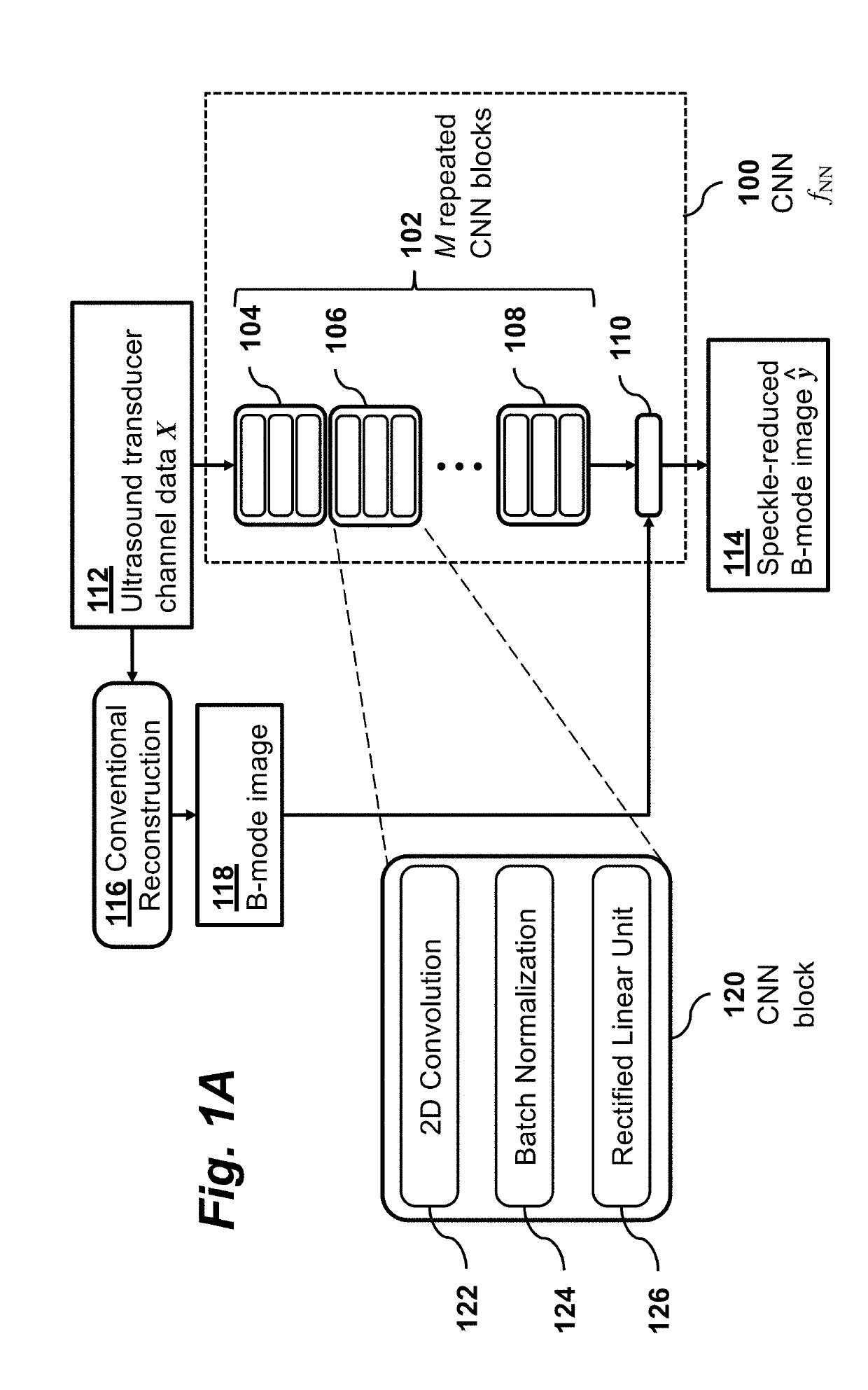
where 1 is an N-vector of ones and |⋅| denotes an element-wise absolute value. According to the present invention, y is estimated by a convolutional neural network using a function ƒNN(X; θ), where θ are the parameters of the network. As illustrated in FIG. 1A, the estimate ŷ=ƒNN(X; θ) is computed by a convolutional neural network 100 that takes the ultrasound transducer data 112 as its input X and produces a speckle-reduced B-mode image 114 as its output ŷ.
[0032]In order to reconstruct desired B-mode images with a neural network, the network 100 is first trained using training data, i.e., a set of inputs and corresponding true outputs that can be compared to the network output using a loss function. The training process is designed to determine the optimal parameters θ* that minimize the error between an estimated image y output from the network and the true image y, as quantified by some loss function (y, ŷ):
θ * = argmin θ ℒ ( y , f NN ( X ; θ ) ) . ( 2 )
The minimization problem is typically solved using some form of gradient descent, an approach in which each of the parameters is iteratively updated to reduce the error:
θ j := θ j - α ∂ ∂ θ j ℒ ( y , f NN ( X ; θ ) ) , ( 3 )
where α denotes the step size, also called the learning rate.
[0033]Standard Loss Functions The choice of loss function significantly affects the training process. The l1 and l2 norms are often used to quantify the reconstruction error:
ℒ 1 ( y , y ^ ) = 1 PQ ∑ p = 1 PQ y p - y ^ p ( 4 ) ℒ 2 ( y , y ^ ) = ( 1 PQ ∑ p = 1 PQ ( y p - y ^ p ) 2 ) 1 2 , ( 5 )
where the p-th pixels of y and ŷ are respectively denoted as yp and ŷp. Alternative metrics such as structural similarity (SSIM) and multi-scale structural similarity (MS-SSIM) have also been proposed. The SSIM between pixels yp and ŷp is computed as
SSIM ( y p - y ^ p ) = ( 2 μ y p μ y ^ p + C 1 μ y p 2 + μ y ^ p 2 + C 1 ) ( 2 σ y p y ^ p + C 2 σ y p 2 + σ y ^ p 2 + C 2 ) , ( 6 )
where C1 and C2 are empirically selected scalar parameters to enhance numerical stability, μy p and μŷ p are the mean values of a neighborhood around yp and ŷp, respectively, σy p 2 and σŷ p 2 are their variances, and σy p ŷ p is their covariance. The means, variances, and covariance are obtained using Gaussian filters. SSIM values range from −1 to 1, where 1 indicates perfect correspondence between the images. Therefore, a loss function can be defined as
ℒ SSIM ( y , y ^ ) = 1 - 1 PQ ∑ p = 1 PQ SSIM ( y p - y ^ p ) . ( 7 )
The MS-SSIM metric extends SSIM by combining SSIM measurements using several neighborhood sizes in order to compare the images at multiple resolution scales. The different scales can be achieved either by downsampling the image or by changing the standard deviation parameter of the Gaussian filter. In this work, we adopt the latter approach.
Loss Functions for Ultrasound B-Mode Imaging
[0034]In B-mode imaging, it is important to accurately reconstruct hypoechoic targets such as blood vessels and heart chambers, whose signals can be more than 40 dB (100 times) weaker than the background tissue. B-mode images are typically compressed prior to being viewed in order to visualize the wide dynamic range. However, the large discrepancy in signal strengths may cause standard loss functions to over-emphasize errors in strongly echogenic targets and to under-emphasize errors in hypoechoic targets. Therefore, we propose to compute losses using logarithmically compressed images, i.e., (log y, log ŷ). This allows the errors to be measured in the same domain that the images are viewed in.
[0035]Another challenge is that B-mode images and their ground truth echogenicity maps are both defined in arbitrary units, making it unclear how to compare the two images. One approach is to normalize each respective image, (e.g., by their maximum values). Unfortunately, the standard loss functions are highly sensitive to the normalization, whereas an ideal loss function for images with arbitrary units should be independent of their normalization.
[0036]Preferred embodiments of the invention use a new loss function that is intrinsically independent of normalization and is suitable for comparing two images with arbitrary units. Let * define the minimum achievable loss when ŷ is scaled by some positive weight parameter w:
ℒ * ( log y , log y ^ ) = min w 0 ℒ ( log y , log w y ^ ) . ( 8 )
These loss functions apply precise normalization to each image such that the 1, 2, and MS-SSIM losses are minimized, respectively, allowing the images to be compared according to their relative contrasts and structures rather than their absolute magnitudes.
[0037]Closed form expressions for the *l 1 , *l 2 , and *MS-SSIM loss functions are provided as follows:
The *l 2 Loss Function
[0038]The optimal weight for the l2-norm is found as:
w 2 * = argmin w 0 y - w y ^ 2 ( 9 ) = argmin w 0 w 2 y ^ T y ^ - 2 w y ^ T y . ( 10 )
The optimum value can be found by taking the derivative with respect to w and solving for the minimum, giving
w 2 * = y ^ T y y ^ T y ^ . ( 11 )
The *l 1 Loss Function
[0039]The optimal weight for the l1-norm is obtained as:
w 1 * = argmin w 0 ∑ p = 1 P w - y p y ^ p . ( 12 )
The minimum, where the derivative with respect to w is zero, can be found by using the relation
∂ ∂ w w - u = sign ( w - u ) , ( 13 )
yielding an optimal solution that is the median value of yp/ŷp:
0 = ∑ p = 1 P sign ( w 1 * - y p y ^ p ) ( 14 ) w 1 * = median { y p y ^ p } p = 1 P . ( 15 )
The *MS-SSIM Loss Function
[0040]The SSIM metric is the product of the differences in luminance, contrast, and structure, which correspond to differences in the mean, standard deviation, and the normalized signals, respectively. When computed on log-images, the optimal weight is additive. In the case of the SSIM, we find that the derivative with respect to w for one pixel p is
∂ ∂ w SSIM ( log y p , w + log y ^ p ) = ( 16 ) 4 μ log y p σ log y p log y ^ p 2 ( μ log y p 2 - ( w + μ log y ^ p ) 2 ) ( σ log y p 2 + σ log y ^ p 2 ) ( μ log y p 2 + ( w + μ log y ^ p ) 2 ) 2 , ( 17 )
where the stabilizing constants C1 and C2 are omitted. The optimal weight is obtained by solving for w over all pixels:
0 = ∑ p = 1 P ∂ ∂ w SSIM ( log y p , w + log y ^ p ) . ( 18 )
Unfortunately, this equation is intractable for large P.
[0041]We instead utilize a (potentially suboptimal) weight:
w * = 1 PQ ∑ p = 1 PQ log y p - 1 PQ ∑ p = 1 PQ log y ^ p . ( 19 )
This is equivalent to computing the SSIM without the luminance term:
SSIM * ( log y p , log y ^ p ) = 1 PQ ∑ p = 1 PQ 2 σ log y p log y ^ p 2 + C 2 σ log y p 2 + σ log y ^ p 2 + C 2 . ( 20 )
Similarly, the multi-scale luminance-independent MS-SSIM loss function is then defined as
ℒ MS - SSIM * ( log y , log y ^ ) = 1 - ∏ j SSIM j * ( log y , log y ^ ) , ( 21 )
where j indexes the scales over which the SSIM* is computed.
Field II Simulation Training Dataset
[0042]The network 100 is preferably trained using simulated ultrasound data. For example, in one embodiment, the Field II Pro simulation package was used to simulate ultrasound channel data from 128 elements of a Verasonics L12-3v linear array transducer. A full synthetic aperture data set was simulated using single-element transmits at 8 MHz with 60% bandwidth. Speckle was simulated with random uniformly distributed scatterers in a 10 mm×10 mm×3 mm phantom centered at the elevation focus of 2 cm. The scatterer density was selected to be 60 scatterers per resolution cell, and the scattering amplitudes were normally distributed and weighted according to ground truth echogenicity maps.
[0043]To provide the network with a wide range of features and contrasts, real photographic images were used as the ground truth echogenicity. The images were taken from publicly available image databases: 512 images from a Places2 test set and 512 images from an ImageNet validation set were selected for a total of 1024 images. These images were used solely for their patterns and contrasts; their corresponding classification labels were not used. The images were converted to grayscale and cropped into a 224 pixel×224 pixel square patch. The patch was then mapped onto the lateral and axial extent of the phantom (10 mm×10 mm) to serve as the ground truth echogenicity map, and the pixel intensities were used to weight the scattering amplitudes of the simulated scatterers according to their positions via bilinear interpolation. This approach was chosen as a convenient alternative to custom-designing a wide variety of ground truth echogenicity maps.
[0044]For each of the 1024 images, an independent set of random scatterers was weighted and used in a full synthetic aperture simulation. For each simulation, the received radiofrequency (RF) channel signals were demodulated and focused into the same 224 pixel×224 pixel grid as the ground truth echogenicity map, with dynamic focusing applied on both transmit and receive. The dimensions of the resulting data cube were 224 pixels×224 pixels×128 channels.
[0045]The set of 1024 simulations was then resampled to generate an augmented training dataset comprised of 5000 co-registered pairs of focused channel data and reference ground-truth echogenicity. The resampled data/reference pairs were selected to have a smaller patch size of 64 pixels×64 pixels and each was drawn randomly from one of the 1024 simulations. While the number of pixels was held constant, the lateral and axial positions and sizes of the patches were allowed to vary independently of one another, resulting in rectangular patches. The resulting 64×64 patches were then treated as though they were square patches with stretched speckle patterns, enabling the emulation of a wide variety of imaging configurations from a limited number of simulations. Each channel dataset was corrupted by a random amount of white thermal noise and band-limited acoustical reverberation noise, specified in decibels (dB) relative to the RMS of the channel signals. Each attribute was selected randomly from a uniform distribution over the range of values listed in Table 1.
TABLE 1 Range of Parameters for Random Patches Attribute Minimum Value Maximum Value Simulation Index 1 1024 Lateral Position −1.9 mm (−10λ) 1.9 mm (10λ) Axial Position 18.1 mm (94λ) 21.9 mm (114λ) Lateral Size 0.4 mm (2λ) 6.2 mm (32λ) Axial Size 0.4 mm (2λ) 6.2 mm (32λ) Thermal Noise −40 dB +6 dB Acoustical Noise −40 dB +6 dB
Image Reconstruction Quality Metrics
[0046]The quality of image reconstruction was measured using several metrics. The *l 1 , *l 2 , and *MS-SSIM errors were computed between the reconstructed log-image and the ground truth echogenicity log-image when available. The *l 2 and *l 1 errors were obtained in units of dB, whereas the *MS-SSIM error was bounded from 0 to 2, with 0 being achieved when y=ŷ. The reconstruction quality was also measured using the contrast and contrast-to-noise ratio (CNR) of cyst targets and using the signal-to-noise ratio (SNR) of the tissue background:
Contrast = 20 log 10 ( μ t μ b ) ( 22 ) CNR = μ t - μ b σ t 2 + σ b 2 ( 23 ) SNR = μ b σ b , ( 24 )
where μt and μb denote the means and σt and σb the standard deviations of the target and background, respectively. Contrast, CNR, and SNR were computed on the linear scale images, prior to log-compression. The CNR essentially combines the contrast and SNR metrics into a single measure of lesion detectability. In the simulations and the phantom, the cyst contrasts and CNRs were measured in concentric regions of interest (ROIs). The target ROI was selected as a circle with a radius of 0.8 times the cyst radius, and the background ROI as a ring with inner and outer radii of 1.1 and 1.5 times the cyst radius, respectively. The background SNR was measured in a homogeneous region of speckle. For DAS beamforming, the measured pixel values in a region of homogeneous echogenicity are classically expected to follow the Rayleigh distribution, resulting in an SNR of 1.91.
[0047]Image resolution was measured using the following methodology. First, the system response to a transition between two regions of different echogenicities was measured, referred to as the edge spread function (ESF). Field II Pro was used to simulate a target wherein half the azimuthal field of view was a speckle region of constant echogenicity and the other half was an anechoic region. The resulting images were averaged axially and over 16 independent scatterer realizations to reduce noise. Next, the ESF was differentiated in the azimuthal dimension to produce a line spread function (LSF). Finally, the FWHM of the LSF was measured to obtain the image resolution.
Deep Convolutional Neural Networks
[0048]Convolutional neural networks were used to estimate echogenicity from the focused and demodulated channel signals. Analysis was restricted to a maximum of 16 channels per pixel due to computational and memory constraints. To achieve this, the 128 element array was subdivided into 16 equal subapertures of 8 elements each, and the signals from each subaperture were beamformed into a single signal, yielding a total of 16 complex signals per pixel. The real and imaginary components were then concatenated in the channel dimension prior to being input into the neural network, resulting in 32 distinct channels per pixel, i.e., for a pixel grid of size P×Q, the resulting data was P×Q×32.
[0049]The network architecture 100 is shown in FIG. 1A. The network 100 has a sequence of M repeated convolution blocks 102, with each block 104, 106, 108 applying a 2D convolution 122, batch normalization 124, and rectified linear unit activation 126. This motif was repeated for all M blocks in the sequence 102. Each 2D convolution layer 122 was composed of F machine-learned filters, and the size of each filter was 7×7×32 for the first layer, 5×5×F for the second layer, and 3×3×F for subsequent layers, with the convolution occurring over the first two dimensions of each. Each convolution was zero-padded in the first two dimensions such that the input and output were the same size, making the size of the output of each convolutional layer P×Q×F.
[0050]The input to the network was a 64×64×32 dataset, where the last dimension corresponded to real and imaginary components of 16 subaperture signals. A conventional DAS envelope-detection reconstruction 116 generates a conventional B-mode image 118, which was concatenated to the output of the M-th block 108. The speckle-reduced B-mode image output 114 was obtained by applying one final 2D convolution 110 and squaring the result. As will be explained further below in relation to FIGS. 4A-C, concatenating the B-mode image 118 after the M-th convolutional block significantly enhances training. Although the input channel data 112 theoretically contain all of the raw information necessary to reconstruct a B-mode image 114, it appears that the concatenated B-mode image 118 served as a good initial estimate of echogenicity for the network to improve upon, rather than learning the reconstruction from scratch. The uncompressed B-mode image 118 is separately formed from the input data 112 using equation (1) and concatenated to the output of the M-th block 108, yielding a data array of size P×Q×(F+1). The final convolution filter 110 of size 1×1×(F+1) was used to produce the output image 114 of size P×Q×1 that was subsequently squared on a pixel-wise basis to yield positive values of echogenicity. The fully convolutional nature of the network allowed echogenicity estimation on a pixel-wise basis. Unless otherwise specified, the default parameters for the networks were M=16 convolution blocks with F=32 filters per layer. Pooling layers and dropout were not utilized.
[0051]In an alternative configuration, the original input is concatenated to the output of one or more of the intermediate blocks instead of the B-mode image, yielding a data array size of 1×1×2F instead of 1×1×(F+1). Any subsequent convolution filters would have the appropriate size (i.e., 2F) to accommodate the new data size. In a different configuration, the network an encoding-decoding structure is used to achieve multi-scale or multi-resolution processing, in which intermediate encoding layers apply pooling or striding, i.e., reduce the data dimensions in the first two dimensions by some factor D, and subsequent intermediate decoding layers increase the data dimensions in the first two dimensions by the same factor D; intermediate layers may be connected via concatenation. In another configuration, the 2D convolution layers are replaced by 3D convolutions that additionally convolve in the transducer channel dimension. In this configuration, the real and imaginary components of the data are preserved as a separate dimension from the channel signals, such that the data size is 64×64×16×2.
[0052]FIG. 1B provides an overview of major components of an apparatus for image reconstruction according to an embodiment of the invention. Transducer array channel signals 150 output from an ultrasound transducer array are provided to ultrasound acquisition hardware 152 which sample, amplify, and digitize the radiofrequency channel signals, which are then provided to signal pre-processing component 154 which performs bandpass filtering, time delays, and demodulation. The pre-processed signals are then input to neural network beamformer 156. The neural network beamformer 156 may be implemented using a GPU, FPGA, ASIC, or other dedicated hardware (e.g., tensor processing unit) to perform the real-time computations associated with the neural network. In a prototype, the neural networks were implemented in Python using TensorFlow using the Adam optimizer with a single NVIDIA GeForce GTX 1080 Ti GPU, which has 11 GB of memory. The output from the neural network 156 is provided to an image processing component 158 which performs compression and persistence, resulting in a final diagnostic image which is presented to a medical professional on an image display 160.
[0053]We performed hyperparameter tuning of the learning rates, batch size, and both l1 and l2 regularization of filter weights to achieve optimal performance using an independent validation dataset that was separate from all other datasets. The final hyperparameters used are tabulated in Table 2.
TABLE 2 Network Training Hyperparameters Hyperparameter Value Learning Rate 1 × 10⁻⁴ Filter l1 Regularization 1 × 10⁻³ Filter l2 Regularization 1 × 10⁻³ Batch Size 128
Neural Network Training and Analysis
[0054]Neural network training performance was analyzed as a function of training objective. A network with 16 convolution blocks and 32 filters per layer was trained to minimize either *l 1 , *l 2 , *MS-SSIM, or a mixture of l1 and MS-SSIM, defined as:
*Mix(y,ŷ)= *l 1 (y,ŷ)+β *MS-SSIM(y,ŷ), (25)
where β was set heuristically to 200 to equalize the contributions of each loss function. Speckle reduction was evaluated on a validation dataset consisting of 32 new Field II Pro simulations, also based on photographs. Performance was quantified using the *l 1 , *l 2 , and *MS-SSIM loss functions. Similarly, speckle reduction performance was also analyzed as a function of depth using networks with 2, 4, 8, or 16 blocks and 32 filters per layer, as well as networks with 16 blocks and 4, 8, 16, or 32 filters per layer, where all of the networks were trained to minimize *Mix. Finally, performance was compared with and without concatenating a B-mode image after the M-th convolution block.
Testing of Speckle Reduction Methods
[0055]All testing was performed using a neural network with a depth of 16 blocks, a width of 32 filters, and trained to minimize the *Mix loss function for 30 training epochs unless otherwise indicated. The speckle reduction performance of the network was compared against those of receive spatial compounding and optimized Bayesian nonlocal means (OBNLM). Spatial compounding was implemented on receive by performing DAS beamforming and envelope detection independently on four non-overlapping subapertures and summing the result. The OBNLM algorithm was applied to images that were beamformed according to equation (1) using the publicly available MATLAB implementation provided by the authors of this algorithm. The default parameter values provided by the authors were used (M=7, α=3, h=0.7).
[0056]Simulation, phantom, and in vivo test datasets were used to evaluate beamforming performance. A simulation test dataset was obtained with Field II Pro with the same imaging configuration as the training dataset. Hypoechoic cylindrical cysts with diameters of 1 mm and 3 mm and contrasts of −20 dB and −6 dB were centered at the elevation focus of 2 cm depth. The full synthetic aperture set of channel signals was retrospectively focused into a 1 cm×1 cm pixel region also centered at the elevation focus, and the channels were delay-and-summed into 16 subaperture IQ signals. The simulated results were assessed using the *l 1 , *l 2 , and *M-SSIM loss functions, as well as contrast, CNR, and SNR.
[0057]Generalizability from simulations to real-world ultrasound data was tested on a CIRS Model 040GSE calibrated phantom imaged using a Verasonics Vantage 256 research scanner with an L12-3v linear array transducer. Single element transmissions at 6 MHz sampled at 24 MHz were used to obtain a full synthetic transmit aperture for dynamic focusing on both transmit and receive. The channel data were focused into a pixel grid of 4 cm in depth and 2 cm in width, with a pixel spacing of λ/2 in both dimensions. Transmit and receive aperture growth were applied to achieve an ƒ-number of 2. The phantom images were evaluated using contrast, CNR, and SNR.
[0058]Generalizability to clinical imaging conditions was assessed in vivo in the kidney of a healthy 58-year-old male volunteer and in the liver of a 68-year-old female who had a focal lesion with a surrounding fluid capsule. Channel datasets were acquired with a modified Siemens S2000 scanner using a Siemens 4C1 transducer. Pulse-inversion harmonic imaging was performed using focused transmissions at 1.82 MHz. Due to technical limitations, the channel signals were obtained for only 64 (out of 192) elements in a sector of 54 (out of 192) beams. The remaining beams were acquired using the full aperture using conventional DAS. The 64 receive channel signals were beamformed into 16 subaperture signals prior to being input into the neural network. For this particular dataset only, a partially-trained network (15 epochs rather than 30) was used to evaluate speckle reduction to avoid overfitting. Image quality was assessed using contrast, CNR, and SNR of the liver lesion vs. the surrounding fluid, with the ROIs selected to obtain a large region of speckle while avoiding obvious and significant changes in underlying echogenicity.
Neural Network Training and Analysis
[0059]FIGS. 2A-C plots the *l 1 , *l 2 , and *MS-SSIM validation losses of neural networks over 50 training epochs for several training objectives, as computed on the validation dataset. The neural network was trained to minimize *MS-SSIM (solid), *l 1 (dashed), *l 2 (dot-dashed), or *Mix (dotted). Performance was measured using the *l 1 (FIG. 2A), *l 2 (FIG. 2B), and *MS-SSIM (FIG. 2C) losses after each training epoch, as measured on the validation dataset. The losses of the DAS reconstruction (thin line) are shown for reference. The networks trained to minimize *l 1 and *Mix were found to yield the lowest *l 1 losses. The networks trained to minimize *MS-SSIM and *Mix yielded the lowest *MS-SSIM and *l 2 losses. Minimizing *l 2 resulted in unstable performance, with erratic increases in all three losses occurring partway through training. Minimizing *Mix resulted in fast and smooth reduction in all three losses.
[0060]FIGS. 3A-F shows the validation losses as a function of network depth and width for a network trained to minimize *Mix on the validation dataset. Given a fixed width of 32 filters, deeper networks converged to lower *l 1 , *l 2 , and *MS-SSIM losses after 50 epochs, and approached these values more rapidly as well. Similar results were observed when fixing the network depth to 16 layers and increasing the width. With the exception of the network with a width of 4 filters, all networks outperformed DAS beamforming by the *l 1 , *l 2 , and *MS-SSIM metrics. In general, it was observed that the deeper and wider networks trained more quickly and resulted in lower *l 1 , *l 2 , and *MS-SSIM losses, as measured on the validation set.
[0061]FIGS. 4A-C plots the same validation losses for networks trained to minimize *Mix with and without a concatenated B-mode image after the M-th convolutional block. The network with B-mode concatenation (solid) significantly outperformed the network without B-mode (dotted) as measured by *l 1 (FIG. 4A), *l 2 (FIG. 4B), and *MS-SSIM (FIG. 4C). The network without B-mode outperformed DAS beamforming in only *MS-SSIM.
[0062]Though not plotted here, the training errors closely followed the trends of the validation errors in all cases in FIGS. 2A-C, FIGS. 3A-F, and FIGS. 4A-C, indicating that the networks were not overfitting to the training data.
Image Resolution
[0063]The FWHM of the LSF was used to measure the azimuthal resolution of each imaging method. The resolutions were found to be: DASFWHM=0.132 mm; SCFWHM=0.156 mm; OBNLMFWHM=0.186 mm; and NNFWHM=0.129 mm, where the neural network was evaluated after being trained to minimize *Mix for 30 epochs.
Cyst Simulation Results
[0064]Images reconstructed using DAS, spatial compounding, OBNLM, and the neural network are pictured in FIG. 5, along with the reference images. Image quality metrics for each method in the test dataset of simulated cysts are presented in Table 3. Overall, the *l 1 and *l 2 losses in the relatively simple test set were lower than those found in the more complex validation set used in FIGS. 2A-C and FIGS. 3A-F, which was composed of photographic images. DAS accurately reproduced contrast in the 3 mm lesions, and was within 3 dB for the 1 mm lesions.
[0065]Qualitatively, spatial compounding exhibited moderate speckle reduction while preserving
TABLE 3 Test Dataset 1: Cyst Simulation Reconstruction Metrics Target Metric DAS SC OBNLM NN* All simulations l 1 ★(dB) 28.09 12.49 4.17 4.88 All simulations l 2 ★(dB) 2.84 1.13 0.20 0.18 All simulations MS-SSIM★ 0.108 0.050 0.005 0.005 −20 dB 1 mm cyst Contrast −17 dB −15 dB −7 dB −13 dB −20 dB 3 mm cyst Contrast −20 dB −19 dB −18 dB −20 dB −6 dB 1 mm cyst Contrast −7 dB −7 dB −2 dB −3 dB −6 dB 3 mm cyst Contrast −6 dB −6 dB −5 dB −5 dB −20 dB 1 mm cyst CNR −1.8 −2.2 −3.6 −4.6 −20 dB 3 mm cyst CNR −1.6 −2.2 −6.5 −6.7 −6 dB 1 mm cyst CNR −1.0 −1.2 −2.4 −2.8 −6 dB 3 mm cyst CNR −0.8 −1.1 −3.1 −2.7 Background SNR 1.87 2.50 11.16 11.00 *Trained to minimize Mix★ for 30 epochs
contrast and resolution throughout the images. Spatial compounding approximately halved the test loss values. The contrast measurements of the −20 dB cyst were slightly worse than DAS, but the SNR was improved by 34%, resulting in overall improvements in CNR. OBNLM applied considerable smoothing to the speckle (497% SNR increase) and produced the lowest *l 1 , losses of all methods. However, OBNLM exhibited a visible loss in resolution, resulting in significantly degraded contrasts in the 1 mm cysts. Note that speckle artifacts are still visible in the background texture of the images, indicating that the smoothing parameter of OBNLM was set conservatively. We observed that relaxing the smoothing parameter resulted in worsened speckle texture without a gain in resolution, while more aggressive smoothing eliminated these artifacts but led to a further loss in resolution (not pictured). Both OBNLM and the neural network resulted in a 20-fold reduction in *MS-SSIM losses from DAS. The neural network additionally had the lowest *l 2 loss of all methods, and increased the speckle SNR by 488%. The neural network resulted in higher CNR than DAS, SC, and OBNLM in all cysts except for the −6 dB 3 mm cyst.
Phantom Imaging
[0066]
TABLE 4 Test Dataset 2: Phantom Reconstruction Metrics Target Metric DAS SC OBNLM NN* −12 dB cyst Contrast −10 dB −10 dB −9 dB −11 dB −6 dB cyst Contrast −5 dB −5 dB −5 dB −5 dB +6 dB cyst Contrast +2 dB +2 dB +2 dB +2 dB +12 dB cyst Contrast +5 dB +5 dB +5 dB +6 dB −12 dB cyst CNR −1.2 −1.6 −2.9 −2.3 −6 dB cyst CNR −0.8 −1.1 −2.2 −1.6 +6 dB cyst CNR +0.2 +0.5 +0.7 +0.8 +12 dB cyst CNR +0.7 +1.2 +2.9 +2.2 Background SNR 1.90 2.57 11.60 7.73 *Trained to minimize Mix★ for 30 epochs
[0067]Images of the tissue mimicking phantom are shown in FIG. 6A-B. The images in FIG. 6A show a −12 dB hypoechoic cyst and a smaller anechoic cyst, while the images in FIG. 6B show a +12 dB hyperechoic cyst and point targets at the top. Contrasts and CNRs for −12 dB, −6 dB (not pictured), +6 dB (not pictured), and +12 dB 8 mm cysts are included in Table 4, along with the speckle SNR. In the DAS images, some mild signal attenuation was visible in the lower half of each image resulting in darker textures. Additionally, both the +6 dB and +12 dB hyperechoic cysts exhibited unexpectedly low contrasts of +1 dB and +5 dB in the DAS image. The DAS speckle SNR of 1.90 matched the classical prediction. Spatial compounding preserved cyst contrasts while smoothing the speckle texture, improving the SNR by 35%. Over the four cysts, spatial compounding improved the CNR on average by 67%. The OBNLM technique significantly smoothed the speckle and preserved the point targets, though the lateral edges of the hypoechoic and anechoic cysts were blurred. Overall, OBNLM improved SNR by 511% and CNR by 211%.
[0068]The neural network demonstrated excellent speckle reduction, improving the SNR by 306% over DAS. The contrasts were also preserved, resulting in higher CNRs than both DAS and spatial compounding in all cases. The neural network images also presented sharp high-resolution outlines around the −12 dB and anechoic cysts, while the outlines around the +12 dB cyst were less sharp. The images were subject to similar attenuation effects as DAS. Some dark textures and structures were visible around the deep cysts, and appeared to correspond to the speckle textures in the DAS image. The three point targets near the transducer surface were also preserved, but were slightly enlarged.
In Vivo Imaging
[0069]
TABLE 5 Test Dataset 3: In Vivo Reconstruction Metrics Target Metric DAS SC OBNLM NN* Liver lesion SNR 1.63 2.62 1.83 3.09 Surrounding fluid Contrast −20 dB −18 dB −19 dB −22 dB Surrounding fluid CNR −1.5 −2.3 −1.6 −2.8 *Trained to minimize Mix★ for 15 epochs
[0070]FIGS. 7A-B are In vivo harmonic B-mode images of a kidney (FIG. 7A) and a complex focal liver lesion surrounded by an anechoic fluid (FIG. 7B). Image quality metrics are included in Table 5. Both spatial compounding images exhibited significantly reduced speckle with marginal losses in resolution in both images. However, there was a visible loss in contrast throughout. The effects combined for a net increase in SNR of 60% and CNR of 56%. OBNLM preserved bright granular structures throughout the brighter regions of tissue but applied aggressive smoothing in darker image regions with gradual changes in echogenicity. Overall, OBNLM increased SNR and CNR over DAS by 12% and by 10%, respectively. The neural network significantly reduced speckle while improving contrast. The structures within the kidney and the lobes of the liver lesion were well-preserved, and the clutter within the surrounding fluid of the liver lesion was reduced. Shadowing effects visible in DAS were preserved in the neural network images. Overall, the SNR and CNR was increased by 90% and 93% over DAS, respectively. FIGS. 7C-D are two additional views of the same kidney and focal liver lesion, with zoomed insets showing closer detail. These figures show substantial speckle reduction with the preservation of fine details and structures.
[0071]In conclusion, the neural network was able to estimate the true echogenicity more accurately than DAS and spatial compounding, as measured by the *l 1 , *l 2 , and *MS-SSIM losses. The neural network beamformer outputted a homogeneous response in regions of constant echogenicity while mostly preserving the shapes of the cysts.
[0072]The neural network is notably trained entirely in silico and can generalize to real-world imaging, including in vivo. The neural network reduced speckle more effectively than receive-only spatial compounding in both the phantom and in vivo. The in vivo results were particularly remarkable considering that the training and test datasets were acquired with a different transducer (L12-3v at 8 MHz vs. 4C1 at 3.6 MHz), imaging configuration (linear vs. curvilinear), and transmit focusing scheme (full synthetic aperture vs. focused transmits), and additionally contained reverberation clutter and inhomogeneities in sound speed leading to focusing errors. The robust performance may be attributed to the wide variety of speckle patterns observed in the randomly generated training dataset. By randomly selecting the physical width, height, and position of each 64×64 pixel training patch, the networks were provided with diverse examples of speckle shapes, which was effectively equivalent to providing the networks with diverse examples of point spread functions. Although the emphasis of this work was placed on the task of estimating echogenicity, the training dataset also contained simulated examples of both white electronic and band-limited acoustic noise, which may have further aided the networks in generalizing to real data.
[0073]The resolution measurements show that the neural network preserves resolution in speckle targets, unlike spatial compounding and OBNLM. Consequently, the network preferably should be trained with not only diffuse scatterers but also sharp point targets. In addition, the training data should be tailored to match the specific imaging parameters (e.g., transducer geometry, frequency, imaging depth, and focusing configuration) of the anticipated applications, including using appropriate speckle-to-pixel size ratios and pixel spacing. In some embodiments, performance may also be improved by explicitly incorporating prior knowledge about the physics of ultrasound beamforming. For example, full spatial compounding on both transmit and receive is known to improve the edge definition of specular targets by interrogating the targets from multiple angles; a hybridized approach with spatial compounding of neural network-beamformed images could potentially yield better visibility of specular boundaries while reducing speckle.
[0074]Overall, the neural networks trained quickly and robustly. All of the presented networks were trained in under 30 minutes on a workstation equipped with a single NVIDIA GeForce GTX 1080 Ti GPU, and could process a single image frame in under 30 ms. The networks converged to nearly identically performing states for random filter weight initializations, indicating good repeatability. The networks were also observed to be insensitive to hyperparameters such as convolution filter weight regularization, which was set to values ranging from 10−4 to 10−1 with marginal differences in output.
[0075]Deeper and wider networks can represent a broader range of functions, a property called expressive power. The benefits of expressive power were shown in FIGS. 3A-F, where the deeper and wider networks were able to lower the *l 1 , *l 2 , and *MS-SSIM losses in the validation dataset more rapidly and to a lower overall value. However, expressive networks are also more prone to overfitting the training data and generalizing poorly to new data. Overfitting can be detected by observing an increase in validation loss during training, and is often caused by a dataset that is too small relative to the expressive power of the network. This type of overfitting was not exhibited in FIGS. 3A-F, which showed stable improvements in validation loss with more training epochs, suggesting that our training dataset was large enough.
[0076]A second form of overfitting can occur when the training dataset distribution differs from the testing dataset distribution, as was the case in this study. The simulated training dataset was obtained using significantly different configurations and noise conditions from the phantom and in vivo test data. Unfortunately, the validation loss could not be used to observe this type of overfitting because the ground truth was unavailable in the phantoms and in vivo. Instead, we qualitatively observed that a network trained for 30 epochs led to less speckle reduction and an over-emphasis of small speckle troughs in vivo as compared to a network trained for just 15 epochs. This suggests that the second form of overfitting occurred, with the network learning to recognize features in the simulated environment that were not present in the in vivo data. Accordingly, in some embodiments, generalizability to in vivo imaging is improved by training the network with more realistic simulations that model full wave propagation to include the effects of phase aberration, reverberation, and attenuation, as well as diffuse, specular, and point reflectors.
[0077]In addition to using a new dataset and reducing the number of training epochs, overfitting can be mitigated by employing regularization. We used the l1- and l2-norms of the filter weights to enforce smaller weights. Furthermore, we utilized a priori knowledge that the backscatter from diffuse scatterers has high correlation coefficients between neighboring array elements to reduce the full 128 element array into 16 beamformed subapertures. Although motivated by computational constraints, subaperture beamforming effectively applied a regularization by reducing the expressivity of the network. More sophisticated forms of regularization, such as total variation, can be included to further reduce the impact of overfitting.
PUM


Description & Claims & Application Information
We can also present the details of the Description, Claims and Application information to help users get a comprehensive understanding of the technical details of the patent, such as background art, summary of invention, brief description of drawings, description of embodiments, and other original content. On the other hand, users can also determine the specific scope of protection of the technology through the list of claims; as well as understand the changes in the life cycle of the technology with the presentation of the patent timeline. Login to view more.