

Method for predicting drop size distribution
a drop size and distribution technology, applied in the field of crude oilwater separation processes, can solve the problems of large drop formation, difficult consistent desalting, and corrosion of heat exchangers
- Summary
- Abstract
- Description
- Claims
- Application Information
AI Technical Summary
Benefits of technology
Problems solved by technology
Method used
Image

Examples
example 1
Batch Simulation
[0033]The first example simulates batch conditions where a constant volume of water-in-oil emulsion is subject to an electric field. The following parameters were chosen:
Density of water, ρw=1.00 g / cc
Density of oil, ρo=0.90 g / cc˜26° API
Viscosity of water=0.1 cP
Electric field intensity=10,000 V / in
Water content=5% by volume
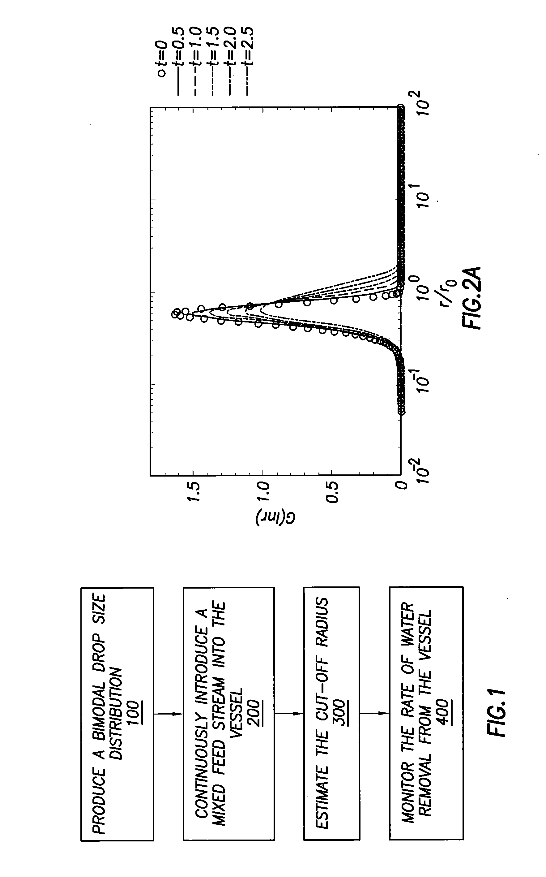
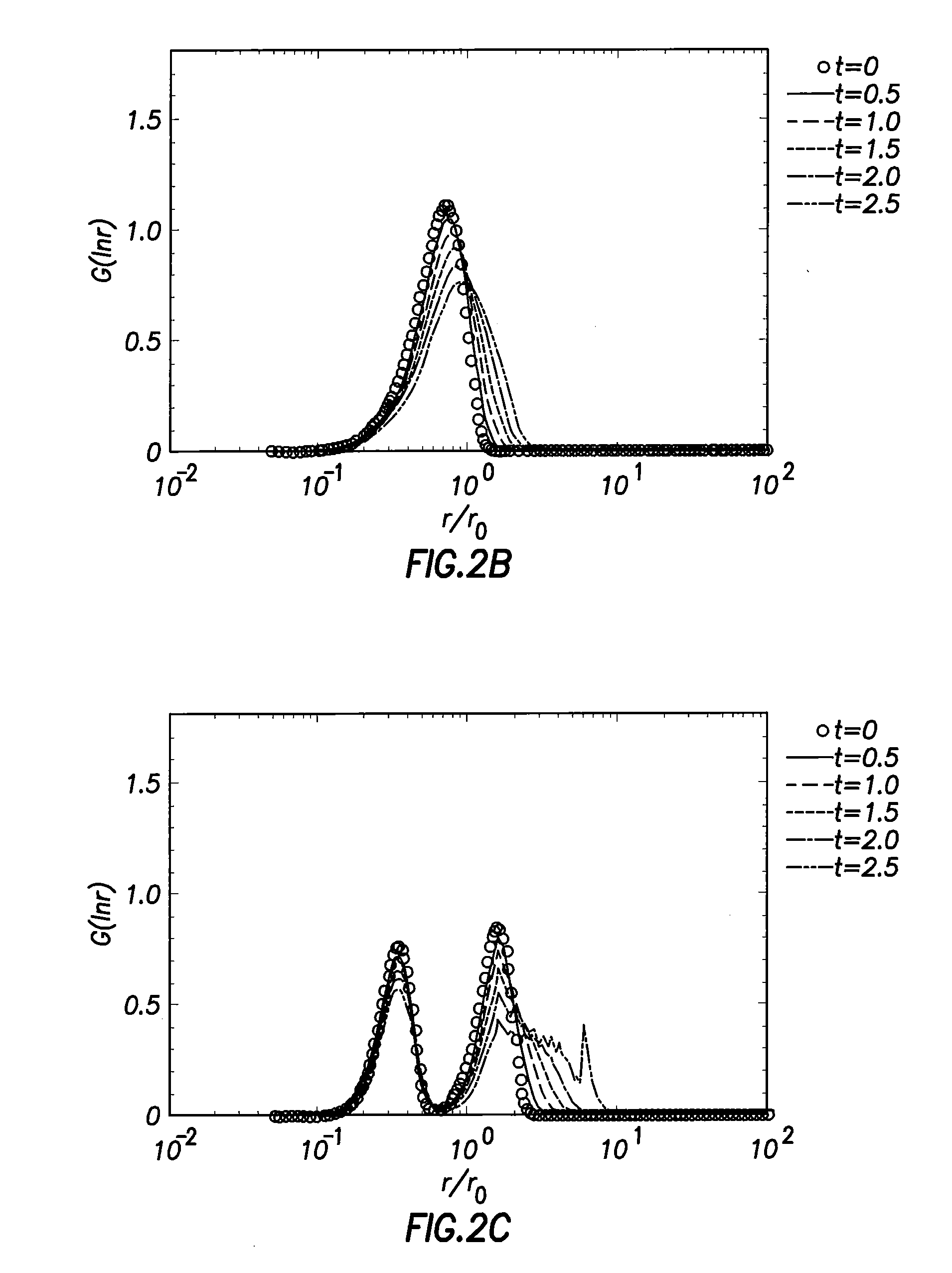
[0034]FIGS. 2(a)-(c) show the evolution of the drop size distribution with time for three different feed conditions. FIGS. 2(a)-(c) show the mass distribution function, G(ln r), plotted as a function of the radius, normalized by an arbitrary radius of ro=50 μm. The open circles correspond to the feed DSD, i.e., DSD at time t=0.
[0035]FIG. 2(c) shows two distinct peaks corresponding to the bimodal distribution. The shifting of the drop size distribution function with time, to larger radii represents drop growth. FIG. 2(c) shows that the peaks decrease in height as the distribution moves to larger sizes since the total mass of water, i.e., the area unde...
example 2
[0039]The second example provides a continuous process with constant feed and outlet stream. The following parameters were chosen:
Density of water, ρw=1.00 g / cc
Density of oil, ρo=0.90 g / cc˜26° API
Viscosity of water=0.1 cP
Electric field intensity=10,000 V / in
Water content=5% by volume
Crude oil flow rate=100,000 bpd
Desalter vessel capacity=7900 ft3
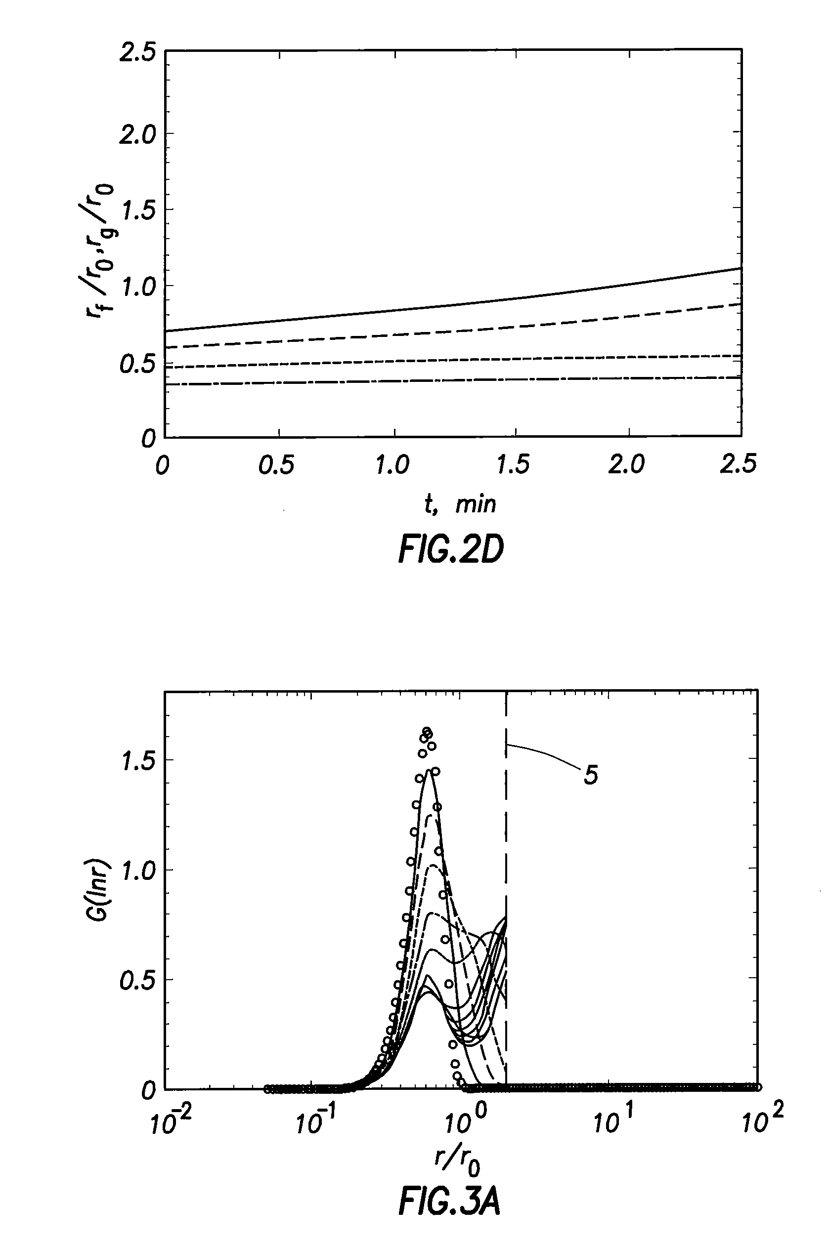
[0040]In these simulations, a constant feed and product crude oil stream are assumed. The amount of water removed is estimated based on the mass of water contained in drops which are larger enough to settle by gravity. A reasonable cut-off radius of rcut=100 μm is assumed. FIG. 3 shows the cut-off radius line 5.
[0041]FIG. 3 shows the evolution of the DSD as a function of time for three feed conditions. The symbols and lines correspond to the feed DSD and DSD plotted in intervals of 1 minute. The total simulation time was 20 minutes. FIG. 3 shows a sharp transition at
r / ro=2,
where the value of the mass distribution functio...
PUM
 Abstract
Description
Claims
Application Information