System and method for extending a lubricant discard interval
- Summary
- Abstract
- Description
- Claims
- Application Information
AI Technical Summary
Benefits of technology
Problems solved by technology
Method used
Image
Examples
example 1
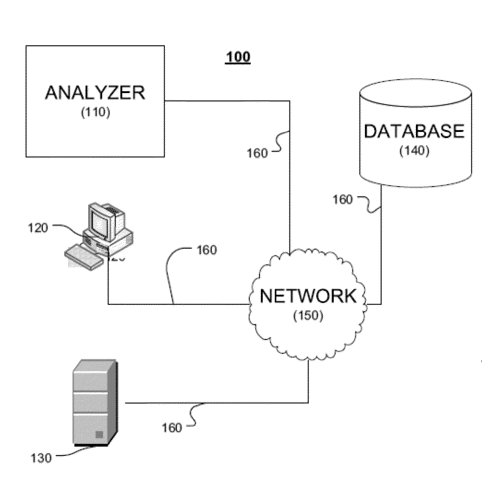
[0115]A locomotive engine is subject to maintenance every 92 days. A sample analysis at 184 indicates that that the oil has 61 days of useful life remaining. The system 100 is used to determine that the useful life can be increased to 92 days by removing 10% of the used oil and replacing with fresh oil. A maintenance manager obtains the output from the system and may then determine whether it is more advantageous to change the oil on that unit at 184 days or draining off 10% of the oil (and adding 10% fresh oil to the unit) and continuing on to 276 days of service before changing the oil.
example 2
[0116]In the following example a partial least squares analysis of data was used to determine when an analysis parameter value would be expected to exceed a threshold value. In the examples, t+X days are arbitrarily selected to illustrate how the analysis is conducted using the claimed system and methods. In the following tables, the values are of each parameter are determined by t+120 days by interpolating between existing data points for each of the measured parameters in a historical record for an engine. For example, Table 1 shows the interpolated values for iron for a particular engine a t+120 days, where t is the estimated oil age in days. Because there is some lag time between when a sample is obtained and the analysis of the sample is determined, the samples are not collected on the last day of a service interval. In other words, the analysis must be received before a selected service interval so that a decision can be made by the time the service interval date arrives. An e...
example 3
[0119]The foregoing analysis can also be done for non-linear data such as viscosity. Table 2 is a table of data for viscosity at 100° C. at t+30 days and t+120 days.
TABLE 2
[0120]FIG. 18 is a scatter plot of observed versus predicted value of viscosity at 100° C. at t+120 days using a partial least squares model with a 3 latent variable model. FIG. 19 is a graphical representation of the amount of variation explained for a 3 latent variable model using the partial least squares model for predicting the viscosity at 100° C. at t+120 days for the data. FIG. 20 is a partial least squares model coefficient chart summary of the three latent variable model depicted in FIG. 19 showing the relative importance / effects of various parameters used for predicting the viscosity at 100° C. at t+120 days. FIGS. 21 and 22 are scatter plots of the multivariate data that was analyzed to predict the interpolated iron content and soot content at t+30 and t+120 days in the oil. The matrix plots also illus...
PUM
 Abstract
Description
Claims
Application Information