Method, device and computer program product for determining an electromagnetic near-field of a field excitation source of an electrical system

Abstract

A method, a device and a computer program product for determining an electromagnetic near-field of a field excitation source of an electrical system are provided, in particular for analysis and / or optimization of an antenna radiation, of a cross-talk problem, of a signal reflexion / transmission, of a stray field, of an irradiation problem or the like. The method includes defining electrical and magnetic properties of the material distribution of the system, defining at least one field excitation source, and determining the electromagnetic near-field components within at least one and in particular all partitions by solution of the Maxwell's equations of the near-field, where each near-field component of each partition can be represented by a linear position of M predetermined ansatz functions Pi orthogonal to one another with regard to a scalar product and weighted with field coefficients vi, and the spatial and / or time derivative of the near-field component can be determined as a linear position of these ansatz functions Pi weighted with derivative coefficients wi, and where each coefficient wi can be determined from a quantity of previously determined field coefficients vi and derivative coefficients wi, so that the determination effort of the near-field of the system rises in substantially linear manner to the number N of partitions in the domain under consideration and to the number M of ansatz functions Pi used in the linear position.

Description

PRIOR ART[0001]The present invention relates to a method, a device and a computer program product for determining an electromagnetic near-field of a field excitation source of an electrical system, in particular for analysis and / or optimization of an antenna radiation, of a cross-talk problem, of a signal reflexion / transmission, of a stray field, of an irradiation problem or the like. In this connection, the electromagnetic system is considered within a domain under consideration split into N partitions.[0002]Methods are known from the prior art for determining an electromagnetic near-field of a field excitation source of an electrical system without application, in particular for optimization of a component development of electromagnetic systems or for optimization of essential electromagnetic properties such as radiation behaviour, beam direction optimization, suppression of cross-talk, optimization of a transmission or reflexion of electromagnetic waves, minimization of a stray f...

AI Technical Summary

Benefits of technology

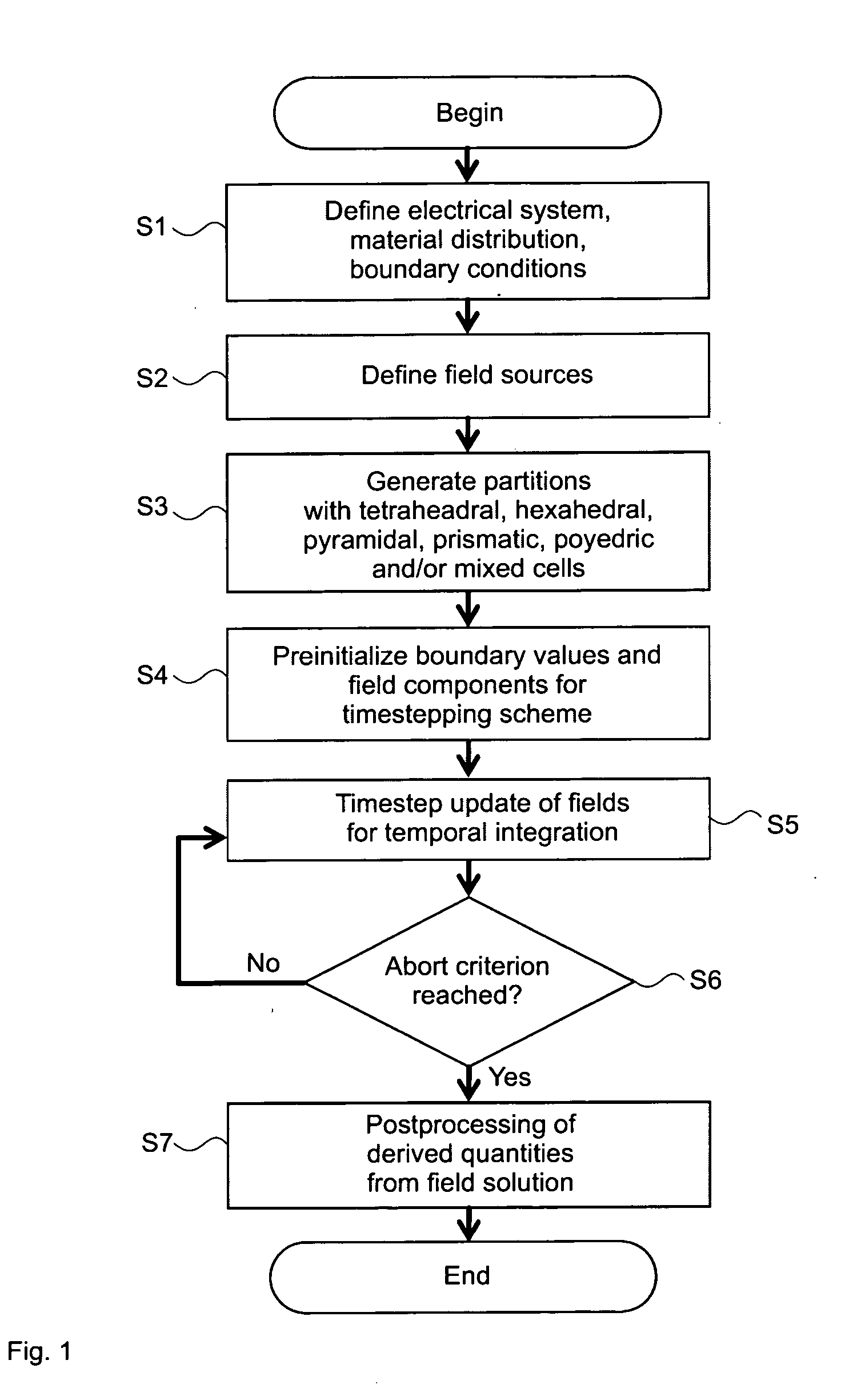
[0025]In accordance with an advantageous embodiment, the domain under consideration is partitioned, i.e. split up into individual grid cells, by an unstructured grid, in particular by a tetrahedral, pyramidal, prismatic grid or by a mixed form of these grid cells, which can for example also comprise hexahedral cells. Unlike a structured grid, an unstructured grid cannot be considered without knowledge of proximity relationships with adjacent grid cells. Structured grids, in particular hexahedral grids or grids in spherical or cylindrical coordinates, permit simple addressing of a grid cell by means of three indices in the three-dimensional case. Unstructured grids, in particular tetrahedral grids, can only be addressed with a greater effort in consideration of a proximity relationship between individual grid nodes, grid surfaces and grid edge. On the other hand, unstructured grids permit a better approximation of geometrical surfaces.

[0032]An explicit integration method permits a simple direct calculation of the field values of a subsequent time step by values of one or more preceding time steps. An implicit method requires for this the solution of an equation system and hence involves a greater determination effort, since a direct update of the field values is not possible. A leapfrog method is a simple method for explicit numerical time integration of an ordinary differential equation by means of physical components offset by half a time step, for example electrical and magnetic field components allocated within a time grid and offset by half a time step. It is thus for example possible to calculate an electrical field strength component Exn+1 at the time (n+1)Δt with time step Δt from a previous electrical field strength component Exn to the previous time step n and from the spatial derivative of a magnetic Hz field strength component to the time step n+1 / 2 withEx(n+1)=Ex(n)+xHz(n+1 / 2).Runge-Kutta methods are based on a truncated Taylor series of a time derivative, where E-field and H-field components can be allocated on the same time grid. By using the leapfrog or Runge-Kutta timestepping method, a transient analysis of an electromagnetic field development can be efficiently performed with linear complexity of the computational effort for the spatial and / or time derivatives in N and M, where the computational effort for the entire problem can grow in superlinear manner up to a fixed end time T thanks to a stability criterion with regard to the time step.

[0037]In accordance with an advantageous further development of the device, the field determination unit is constructed to determine at least one and in particular all electromagnetic near-field components by means of a DG-FEM method (Discontinuous Galerkin Finite Element Method). A DG-FEM method for calculation of electromagnetic fields using orthogonal ansatz functions, whose weighting coefficients can be determined in linearly recursive manner from predetermined weighting coefficients, allows an efficient determination of electromagnetic fields with substantially linear complexity of the number N of partitions and, regardless of this, substantially linear complexity with regard to the number M of used ansatz functions Pi.

[0052]The method achieves, thanks to an implicit and fast application of the operators involved (gradient, trace and their transposes, and the mass operators and their inverses) enhanced efficiency with regard to storage requirements and computation time on hexahedral, prismatic, pyramidal and tetrahedral elements. This represents the central component of the method. For each grid element, only auxiliary quantities are stored and the operators do not have to be explicitly set up as matrices. This permits complexity reduction of the storage requirement. By the use of hierarchical orthogonal ansatz functions (Legendre or Jacobi polynomials) with tensor structure (e.g. Dubiner ansatz on the tetrahedrons [2]) and covariant transformation to reference elements, the complexity of the runtime for the method is reduced. In the three-dimensional case, storage requirement and runtime of the algorithm possess the complexity O(p3) for non-curved elements with cell-constant and field-independent material coefficients and O(p4) for curved elements and / or variable and / or field-dependent material coefficients (i.e. non-linear material laws). p designates the polynomial degree of the method. Absolute runtimes and storage requirement are set forth in the calculation examples further below. For non-curved elements, the result is thus a linear complexity; for the curved elements applied only in special cases in part-areas, the result is a considerably less than quadratic complexity.

[0062]The geometrical independence of the curl and trace operators is achieved by use of a covariant transformation of the ansatz and test functions of any elements from the function spaces of the reference elements, as described for example in [1 p. 331ff]. The following describes the core of the method, fast application of the curl and trace operators and their transposes for the grid elements. Recursion formulas for hierarchical orthogonal Jacobi polynomials were developed and used, which reduce the complexity of the storage requirement and of the application of the curl and trace operators and their transposes to O(p3).Curl Operator

Problems solved by technology

However, at present only methods are known which require a complex inversion of a global equation system and have—in particular in the case of an increase of the polynomial degree p—a superlinear determination complexity.

These methods are thus unsuitable for electromagnetically large domains under consideration.

The drawback of a discretization of electromagnetic systems by means of structured cells is the lack of flexibility in grid generation, where in particular curved surfaces of components or structures can only be imaged with great difficulty using structured grids.

Unstructured grids permit a substantially better imaging of curved surfaces of electromagnetic systems, however the greater computational effort required for the same size of domain under consideration sets natural limits on the complexity of an electromagnetic system.

An application of the method leads not to a linear, but to an at least quadratic numerical complexity in the case of an increase of the polynomial degree.

The prior art thus results in the problem of providing a determination method for analysis and optimization of an electrical system, in particular in respect of an antenna radiation, of a cross-talk problem, of a signal reflexion or transmission, of determination of a stray field (RCS—Radar Cross Section calculation), of an antenna radiation or similar, using which method the Maxwell's equations can be solved on an unstructured, in particular tetrahedral, pyramidal, prismatic or mixed grid, whereby the computational effort grows linearly with the number of unknowns to be determined in the domain under consideration, i.e. linearly with regard to the number of partitions N (h-refinement) and linearly with the number M of ansatz functions used, in particular affected by the approximation quality of the ansatz functions (p-refinement).

Images